Exploring and Analyzing LC-MS Data with Spectra and xcms
Philippine Louail, Johannes Rainer
Eurac Research, Bolzano, Italy; johannes.rainer@eurac.edu github: jorainerFebruary 2024
Source:vignettes/xcms-preprocessing.Rmd
xcms-preprocessing.RmdAbstract
In this document we discuss liquid chromatography (LC) mass
spectrometry (MS) data handling and exploration using the MsExperiment
and r Biocpkg("Spectra") Bioconductor packages and perform
the preprocessing of a small LC-MS data set using the xcms package
(Louail et al. 2025). Functionality from
the MetaboCoreUtils
and MsCoreUtils
packages are used for general tasks frequently performed during
metabolomics data analysis. Ultimately, the functionality from these
packages can be combined to build custom, data set-specific (and
reproducible) analysis workflows.
In the present workshop, we first focus on data import, access and visualization which is followed by the description of a simple data centroiding approach and finally we present an xcms-based LC-MS data preprocessing that comprises chromatographic peak detection, alignment and correspondence. Data normalization procedures, compound identification and differential abundance analysis are not covered here. Particular emphasis is given on deriving and defining data set-dependent values for the most critical xcms preprocessing parameters.
Introduction
Preprocessing is the first step in the analysis of untargeted LC-MS or gas chromatography (GC)-MS data. The aim of the preprocessing is the quantification of signals from ions measured in a sample, adjusting for any potential retention time drifts between samples followed by the matching of the quantified signal across samples within an experiment. The resulting two-dimensional matrix with abundances of the so called LC-MS features in all samples can then be further processed, e.g. by normalizing the data to remove differences due to sample processing, batch effects or injection order-dependent signal drifts. LC-MS features are usually only characterized by their mass-to-charge ratio (m/z) and retention time and hence need to be annotated to the actual ions and metabolites they represent. Data normalization and annotation are not covered by this tutorial but links to related tutorials and workshops are provided at the end of the document.
Mass spectrometry
Mass spectrometry allows to measure abundances of charged molecules (ions) in a sample. Abundances are determined as ion counts for a specific mass-to-charge ratio m/z. The measured signal is represented as a spectrum: intensities along m/z.
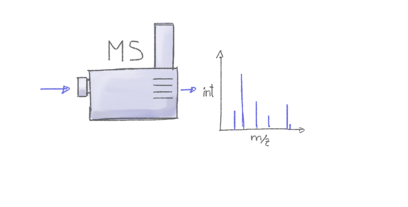
Many ions will result, when measured with MS alone, in a very similar m/z. Thus, making it difficult or impossible to discriminate them. MS is therefore frequently coupled with a second technology to separate ions prior quantification based on properties other than their mass (e.g. based on their polarity). Common choices are gas chromatography (GC) or liquid chromatography (LC). In a typical LC-MS setup a sample gets injected into the system, the molecules in the sample are separated in the LC column, get ionized and then measured (at discrete time points) by the MS instrument (see Figure below for a simple visualization). Molecules get thus separated on two different dimensions, the retention time dimension (from the LC) and the mass-to-charge dimension (from the MS) making it easier to measure and identify molecules in more complex samples.
In such GC/LC-MS based untargeted metabolomics experiments, the data is analyzed along the retention time dimension and chromatographic peaks (which are supposed to represent the signal from ions of a certain type of molecule) are quantified.
Goals of this workshop
Learn how R/xcms and the packages from the RforMassSpectrometry initiative can be used to inspect, evaluate and analyze LC-MS data.
Learn the basis to build reproducible analysis workflows, tailored and customized for individual data sets.
Definitions and common naming convention
Naming conventions and terms used in this document are:
- chromatographic peak: peak containing the signal from an ion in retention time dimension (different from a mass peak that represents the signal along the m/z dimension within a spectrum).
- chromatographic peak detection: process in which chromatographic peaks are identified within a sample (file).
- alignment: process that adjusts for retention time differences (i.e. possible signal drifts from the LC) between measurements/samples.
- correspondence: grouping of chromatographic peaks (presumably from the same ion) across samples/files into LC-MS features.
- feature (or LC-MS features): entity representing signal from the same type of ion/molecule, characterized by its specific retention time and m/z. In xcms, features represent identified chromatographic peaks grouped across samples/files.
Data import and exploration
The example data set of this workflow consists of two files in mzML format with signals from pooled human serum samples measured with a ultra high performance liquid chromatography (UHPLC) system (Agilent 1290) coupled with a Q-TOF MS (TripleTOF 5600+ AB Sciex) instrument. Chromatographic separation was based on hydrophilic interaction liquid chromatography (HILIC) separating metabolites depending on their polarity. The input files contain all signals measured by the MS instrument (so called profile mode data). To reduce file sizes, the data set was restricted to an m/z range from 105 to 134 and retention times from 0 to 260 seconds. Both QC pool samples were taken from a larger experiment and were injected in the same measurement run at different time points (injected in position 1 and 19 of the measurement run).
In the code block below we first load all required libraries and
define the location of the mzML files, which are distributed through the
msdata R package. We also define a data.frame with
the names of the mzML files, an arbitrary sample name, the index in
which the respective sample was measured within the LC-MS run and the
sample group of the samples. It is generally suggested to
provide all experiment-relevant phenotypic and technical information
through such a data frame. Also, the data frame could be defined in an
xls sheet that could then be imported with the read_xlsx
function from the readxl R package. This data frame is then
passed, along with the file names, to the
readMsExperiment() call to import the data.
#' Load required libraries
library(xcms)
library(MsExperiment)
library(Spectra)

#' Define the file names.
fls <- dir(system.file("sciex", package = "msdata"), full.names = TRUE)

#' Define a data.frame with additional information on these files.
pd <- data.frame(file = basename(fls),
                 sample = c("POOL_1", "POOL_2"),
                 injection_index = c(1, 19),
                 group = "POOL")

#' Import the data of the experiment
mse <- readMsExperiment(fls, sampleData = pd)
mse
## Object of class MsExperiment
## Spectra: MS1 (1862)
## Experiment data: 2 sample(s)
## Sample data links:
## - spectra: 2 sample(s) to 1862 element(s).The MS data of the experiment is now represented by an
MsExperiment object.
Basic data access
The MsExperiment object manages the linkage
between samples and spectra. The length() of an
MsExperiment is defined by the number of samples (files)
within the object.
#' Number of samples
length(mse)
## [1] 2Subset the MsExperiment will restrict (all) data within
the object to the selected sample(s). To restrict to data from the
second sample we use:
#' Subset the data
mse_2 <- mse[2]
mse_2
## Object of class MsExperiment
## Spectra: MS1 (931)
## Experiment data: 1 sample(s)
## Sample data links:
## - spectra: 1 sample(s) to 931 element(s).This did subset the full data, including sample information and
spectra data to those of the second file. Phenotype information can be
retrieved with the sampleData() function from an
MsExperiment object.
#' Extract sample information
sampleData(mse_2)
## DataFrame with 1 row and 5 columns
## file sample injection_index
## <character> <character> <numeric>
## 20171016_POOL_POS_3_105-134.mzML 20171016_P... POOL_2 19
## group spectraOrigin
## <character> <character>
## 20171016_POOL_POS_3_105-134.mzML POOL /usr/local...The MS data is stored as a Spectra object within the
MsExperiment and can be accessed using the
spectra() function.
#' Access the MS data
spectra(mse)
## MSn data (Spectra) with 1862 spectra in a MsBackendMzR backend:
## msLevel rtime scanIndex
## <integer> <numeric> <integer>
## 1 1 0.280 1
## 2 1 0.559 2
## 3 1 0.838 3
## 4 1 1.117 4
## 5 1 1.396 5
## ... ... ... ...
## 1858 1 258.636 927
## 1859 1 258.915 928
## 1860 1 259.194 929
## 1861 1 259.473 930
## 1862 1 259.752 931
## ... 34 more variables/columns.
##
## file(s):
## 20171016_POOL_POS_1_105-134.mzML
## 20171016_POOL_POS_3_105-134.mzMLFrom version 4 on, xcms supports the more modern and flexible infrastructure for MS data analysis provided by the Spectra package. While it is still possible to use xcms together with the MSnbase package, users are advised to switch to the newer infrastructure as it provides more flexibility and a higher performance. Also, through additional packages such as the MsBackendRawFileReader, the new infrastructure would allow to import MS data also from other files than mzML, mzXML or CDF files.
In the next few examples we briefly explain the Spectra
object and illustrate the use of such objects using some simple
examples. More information on Spectra objects can be found
in the package’s documentation
or the SpectraTutorials.
The Spectra object contains the full MS data of the
experiment. It’s length is thus equal to the total number of spectra
within the experiment. Below we determine this number for our example
data set. To avoid nested function calls and hence improve the
readability of the code, we use the R pipe operator |>
that allows to concatenate consecutive calls in a more readable
fashion.
## [1] 1862The Spectra object itself is agnostic of any sample
information, it simply contains all spectra from the experiment, first
all spectra from the first file, followed by the spectra from the
second. The mapping of spectra to samples is defined in the
MsExperiment object. To access spectra from a specific
sample we either subset the MsExperiment to that particular
sample (as done in the example above) or we use the
spectraSampleIndex() function that returns for each
spectrum the index of the file within the MsExperiment to
which it belongs. Below we use spectraSampleIndex() to
determine the total number of spectra per sample.
#' Get the number of spectra per file.
spectraSampleIndex(mse) |>
    table()
##
## 1 2
## 931 931Such basic data summaries can be helpful for a first initial quality assessment to identify potentially problematic data files with e.g. a unexpected low number of spectra.
Besides the peak data (m/z and intensity values) also
additional spectra variables (metadata) are available in a
Spectra object. These can be listed using the
spectraVariables() function that we call on our example MS
data below.
#' List available spectra variables
spectra(mse) |>
    spectraVariables()
## [1] "msLevel" "rtime"
## [3] "acquisitionNum" "scanIndex"
## [5] "dataStorage" "dataOrigin"
## [7] "centroided" "smoothed"
## [9] "polarity" "precScanNum"
## [11] "precursorMz" "precursorIntensity"
## [13] "precursorCharge" "collisionEnergy"
## [15] "isolationWindowLowerMz" "isolationWindowTargetMz"
## [17] "isolationWindowUpperMz" "peaksCount"
## [19] "totIonCurrent" "basePeakMZ"
## [21] "basePeakIntensity" "electronBeamEnergy"
## [23] "ionisationEnergy" "lowMZ"
## [25] "highMZ" "mergedScan"
## [27] "mergedResultScanNum" "mergedResultStartScanNum"
## [29] "mergedResultEndScanNum" "injectionTime"
## [31] "filterString" "spectrumId"
## [33] "ionMobilityDriftTime" "scanWindowLowerLimit"
## [35] "scanWindowUpperLimit"Thus, for all spectra we have general information such as the MS
level ("msLevel") or the retention time
("rtime") available. For most of these spectra variables
dedicated accessor functions are available (such as
msLevel, rtime). In addition it is possible to
access any variable using $ and the name of the variable
(similar to accessing the columns of a data.frame). As an
example we extract below the msLevel spectra variable and
use the table() function on the result to get an overview
of the number of spectra from different MS levels available in the
object.
##
##    1
## 1862
The present data set contains thus 1,862 spectra, all from MS level 1.
We could also check the number of peaks per spectrum in the different
data files. The number of peaks per spectrum can be extracted with the
lengths() function. Below we extract these values, split
them by file and then calculate the quartiles of the peak counts using
the quantile() function.
#' Get the distribution of peak counts per file
spectra(mse) |>
    lengths() |>
    split(fromFile(mse)) |>
    lapply(quantile)
## $`1`
## 0% 25% 50% 75% 100%
## 456.0 1122.5 1536.0 2089.0 3995.0
##
## $`2`
## 0% 25% 50% 75% 100%
## 481.0 1101.5 1557.0 2153.5 4088.0Thus, for the present data set, the number of spectra and also the average number of peaks per spectra are comparable.
Individual MS spectra can be accessed by subsetting the
Spectra object returned by spectra(). As an
example we below subset the data to the second sample, extract the
spectra from that sample and subset to the spectrum number 123.
#' Extract one spectrum from the second file
sp <- spectra(mse[2])[123]
sp
## MSn data (Spectra) with 1 spectra in a MsBackendMzR backend:
## msLevel rtime scanIndex
## <integer> <numeric> <integer>
## 1 1 34.314 123
## ... 34 more variables/columns.
##
## file(s):
## 20171016_POOL_POS_3_105-134.mzMLm/z and intensity values can be extracted from a
Spectra using the mz() and
intensity() functions that (always) return a list of
numeric vectors with the respective values:
#' Extract m/z values
mz(sp)
## NumericList of length 1
## [[1]] 105.95354942709 105.955001209814 ... 133.105299625013 133.106926815539
#' Extract intensity values
intensity(sp)
## NumericList of length 1
## [[1]] 0 282 0 141 0 0 141 0 141 0 141 0 ... 563 563 422 0 0 282 282 0 282 141 0As an alternative, the peaksData() function could be
used to extract both the m/z and intensity values (as
two-column numeric matrix) with a single function call.
The total ion signal of a spectrum could be calculated by simply summing the intensities of all peaks in the spectrum. Below we perform that operation on the spectrum extracted above.
## [1] 604912The same operation can also be applied to the full data set. As an
example we calculate below the total ion signal for each spectrum in the
first file and determine the distribution of these using the
quantile() function.
#' Calculate the distribution of total ion signal of the first file
mse[1] |>
    spectra() |>
    intensity() |>
    sum() |>
    quantile()
## 0% 25% 50% 75% 100%
## 69074.0 445575.5 697201.0 897149.5 1562795.0We repeat the operation for the second file.
##        0%       25%       50%       75%      100%
##   70414.0  404923.5  674512.0  878191.0 1679901.0
The total ion signals of the two data files is (as expected) similar.
Through the Spectra object we have thus the possibility to
inspect and explore the (raw) MS data of an experiment and use its
functionality to create own quality assessment functions. Alternatively,
also the MsQuality
package (Naake et al. 2023) could be used
to calculate core MS quality metrics on a full experiment
(MsExperiment) or individual data files
(Spectra).
Data visualization
General data overview
Visualization is crucial for quality assessment of MS data. For LC-MS
data visualizing a base peak chromatogram (BPC) or total ion
chromatogram (TIC) would for example allow to evaluate the performance
of the liquid chromatography of the various samples in an experiment. To
create such a plot we below extract the BPC from our data. The BPC
extracts the maximum peak signal from each spectrum in a data file and
allows thus to plot this information (on the y-axis) against the
retention time for that spectrum. While we could also extract these
values similarly to the total ion intensity in the previous section, we
use below the chromatogram() function that allows
extraction of chromatographic data from MS data (e.g. from an
MsExperiment object). With parameter
aggregationFun = "max" we define to report the maximum
signal per spectrum (setting aggregationFun = "sum" would
in contrast sum up all intensities of a spectrum and hence return a
TIC).
#' Extract and plot a BPC
bpc <- chromatogram(mse, aggregationFun = "max")
plot(bpc)
This plot shows the BPC for each of the two data files (each line representing one sample) and provides the information at what retention times signal was measured (thus at what retention times compounds eluted from the LC column). We can clearly spot regions along the retention time in which more signal/compounds eluted. Also, the BPC of the two data files look similar, which is expected since both represent the same sample.
In addition to a visual inspection it is, especially for larger data sets, important to also quantitatively compare the data and derive quality metrics of a data set. For our base peak signals, however, retention times will be slightly different between the samples preventing thus a direct comparison and evaluation of this data. An easy solution to this is to bin the data along the retention time axis into equal sized bins and aggregate the measured intensities within each bin (per sample). Below we bin the data with a bin size of 1 second reporting the maximal signal per bin.
#' Bin the BPC
bpc_bin <- bin(bpc, binSize = 1)
After binning, the two chromatograms have the same retention times
(and number of intensities) and we can thus bind their
intensity vectors as columns of a new numeric matrix using
cbind():
We could now for example calculate the correlation between the intensities of the two samples, which can be used as a measure for the similarity of the LC-MS runs.
#' Assess similarity between the numerical vectors using a simple
#' Pearson correlation.
cor(bpc_mat[, 1], bpc_mat[, 2])
## [1] 0.9605883We could also create a correlation matrix with the pairwise correlation coefficients of all samples against all samples. This would be particularly helpful for data sets with more than two samples.
#' Create a pairwise correlation matrix
cor(bpc_mat)
## [,1] [,2]
## [1,] 1.0000000 0.9605883
## [2,] 0.9605883 1.0000000Such a correlation matrix could also be easily visualized as a heatmap - with the additional possibility to cluster samples with similar BPC. While for the present, two-sample data set, this is not very informative, for larger data sets it can help to evaluate differences between batches or to spot outlier samples (or rather outlier LC-MS measurement runs).

Heatmap for similarity of the BPC of the two data files
This also exemplifies the power of an R-based analysis workflow that allows us to combine LC-MS specific analysis methods provided by e.g. the xcms package with build-in R functions or (statistical) data analysis methods provided by any other R package.
The BPC collapsed the 3-dimensional LC-MS data (m/z by retention time by intensity) into 2 dimensions (retention time by intensity). An orthogonal visualization to this would be a base peak spectrum (BPS) that collapses the data in retention time dimension. Such a visualization could provide information on the most abundant masses (or rather mass-to-charge values) in the data set (regardless of the retention time in which they were measured). In contrast to the BPC it is however not straight forward to create such a visualization: mass peaks, even if representing signal from the same ion, will never be identical between consecutive spectra, but will slightly differ based on the measurement error/resolution of the instrument.
Below we plot the spectra for 2 consecutive scans.
#' Plot two consecutive spectra
plotSpectra(spectra(mse)[123:124], xlim = c(105, 130))
Spectra from two consecutive scan of the first file
These two spectra could now be merged by reporting for each
m/z (or rather for peaks with very similar m/z in
consecutive spectra) the maximal signal observed. In Spectra,
the combineSpectra() function allows to aggregate/combine
sets of spectra into a single spectrum. By default, this function will
combine sets of spectra (that can be defined with parameter
f) creating an union of the peaks present in spectra of a
set. For mass peaks with a similar m/z value (depending on
parameter ppm) the peaks’ intensities are aggregated using
the function defined with parameter intensityFun to result
in a single value per (aggregated) peak. With the setting below we
combine all spectra from one file (by using
f = fromFile(mse)) into a single spectrum containing mass
peaks present in any of the spectra of that file. Mass peaks with a
difference in their m/z that is smaller than ppm
(parts-per-million of the m/z value) are combined into one peak
for which the maximal intensity of the grouped peaks is reported. Note
that it is suggested to use a small value for ppm to
combine MS1 spectra with combineSpectra().
#' Combine all spectra of one file into a single spectrum
bps <- spectra(mse) |>
    combineSpectra(f = fromFile(mse), ppm = 5, intensityFun = max)
bps
## MSn data (Spectra) with 2 spectra in a MsBackendMemory backend:
## msLevel rtime scanIndex
## <integer> <numeric> <integer>
## 1 1 0.280 1
## 2 1 0.275 1
## ... 34 more variables/columns.
## Processing:
## Switch backend from MsBackendMzR to MsBackendMemory [Fri Dec 12 08:40:51 2025]
## Switch backend from MsBackendMzR to MsBackendMemory [Fri Dec 12 08:40:53 2025]
## Merge 2 Spectra into one [Fri Dec 12 08:40:53 2025]bps is thus a Spectra with two spectra
representing the BPS of the two data files. Below we plot these.
#' Plot the BPS
plotSpectra(bps)
Base peak spectrum for each of the two samples.
These BPS thus show the most common ions present in each of the two samples. Apparently there seems to be quite some overlap in ion content between the two files. Also here, we can calculate similarities between these spectra. As before, we could either bin the spectra and calculate a correlation matrix between their intensities:
#' Bin the spectra and calculate similarity between their intensities
bps_bin <- bin(bps, binSize = 0.01)

do.call(cbind, intensity(bps_bin)) |>
    cor()
## [,1] [,2]
## [1,] 1.0000000 0.9898653
## [2,] 0.9898653 1.0000000Alternatively, we can also directly calculate the similarity between
the base peak spectra using the compareSpectra() function
and one of the available peak similarity measures. Below we use the
normalized dot product to calculate the similarity between the two
spectra matching peaks using an m/z tolerance of 10 ppm.
#' Calculate normalized dot product similarity between the spectra
compareSpectra(bps, ppm = 10, FUN = MsCoreUtils::ndotproduct)
## 1 2
## 1 1.0000000 0.9803889
## 2 0.9803889 1.0000000These measures thus allow us to get some general information on a data set and evaluate similarities between the samples of an experiment.
Detailed data inspection
Apart from such general data overview it is also possible (and also
suggested) to explore the data in more detail. To this end we next focus
on a specific subset of the data were we expect signal for a compound
that should be present in serum samples (such as ions of the molecule
serine). With the particular LC-MS setup used for the present samples,
ions for this metabolite are expected to elute at about 180 seconds
(this retention time was determined by measuring a pure standard for
this compound on the same LC-MS setup). We thus filter below the spectra
data using the filterRt() function extracting only spectra
measured between 180 and 181 seconds.
#' Extract all spectra measured between 180 and 181 seconds
sps <- spectra(mse) |>
    filterRt(c(180, 181))
sps
## MSn data (Spectra) with 6 spectra in a MsBackendMzR backend:
## msLevel rtime scanIndex
## <integer> <numeric> <integer>
## 1 1 180.240 646
## 2 1 180.519 647
## 3 1 180.798 648
## 4 1 180.235 646
## 5 1 180.514 647
## 6 1 180.793 648
## ... 34 more variables/columns.
##
## file(s):
## 20171016_POOL_POS_1_105-134.mzML
## 20171016_POOL_POS_3_105-134.mzML
## Processing:
## Filter: select retention time [180..181] on MS level(s) [Fri Dec 12 08:40:54 2025]For the present data set there are 6 spectra measured within this one
second in both samples. By extracting the data as a Spectra
object we have however lost now the direct (inherent) association
between spectra and samples of the experiment. We could extract the name
of the original data file from which the data was imported (see example
below) and use that to determine the originating sample, but that would
involve additional R code.
#' List the original data file for each spectrum
basename(dataOrigin(sps))
## [1] "20171016_POOL_POS_1_105-134.mzML" "20171016_POOL_POS_1_105-134.mzML"
## [3] "20171016_POOL_POS_1_105-134.mzML" "20171016_POOL_POS_3_105-134.mzML"
## [5] "20171016_POOL_POS_3_105-134.mzML" "20171016_POOL_POS_3_105-134.mzML"Alternatively, we could use the filterSpectra() function
on the MsExperiment object passing the filter function (in
our case filterRt()) to that function. This filters the
Spectra object within the
MsExperiment retaining all associations (links) between
samples and subset spectra. While some of the most commonly used filter
functions, such as filterRt() or
filterMsLevel(), are also implemented for
MsExperiment, the filterSpectra() function
allows to apply any of the many filter functions available for
Spectra objects to the data.
#' Subset the whole MsExperiment
mse_sub <- filterSpectra(mse, filter = filterRt, rt = c(180, 181))
#' Extract spectra from the subset for the first sample
spectra(mse_sub[1])
## MSn data (Spectra) with 3 spectra in a MsBackendMzR backend:
## msLevel rtime scanIndex
## <integer> <numeric> <integer>
## 1 1 180.240 646
## 2 1 180.519 647
## 3 1 180.798 648
## ... 34 more variables/columns.
##
## file(s):
## 20171016_POOL_POS_1_105-134.mzML
## Processing:
## Filter: select retention time [180..181] on MS level(s) [Fri Dec 12 08:40:55 2025]For the present purpose it is however not important to keep the sample association intact and we thus proceed to plot the previously extracted spectra.
#' Plot the spectra
plotSpectra(sps)
MS1 spectra measured between 180 and 181 seconds
We can immediately spot several mass peaks in the spectrum, with the
largest one at an m/z of about 130 and the second largest at
about 106, which could represent signal for an ion of Serine. Below we
calculate the exact (monoisotopic) mass for serine from its chemical
formula C3H7NO3 using the calculateMass() function
from the MetaboCoreUtils
package.
#' Calculate the (monoisotopic) mass of serine
library(MetaboCoreUtils)
mass_serine <- calculateMass("C3H7NO3")
mass_serine
## C3H7NO3
## 105.0426The native serine molecule is however uncharged and can thus
not be measured by mass spectrometry. In order to be detectable,
molecules need to be ionized before being injected in an MS instrument.
While different ions can (and will) be generated for a molecule, one of
the most commonly generated ions in positive polarity is the
[M+H]+ ion (protonated ion). To calculate the m/z
values for specific ions/adducts of molecules, we can use the
mass2mz() function, also from the MetaboCoreUtils
package. Below we calculate the m/z for the [M+H]+ ion
of serine providing the monoisotopic mass of that molecule and
specifying the adduct we are interested in. Also other types of adducts
are supported. These could be listed with the adductNames
function (adductNames() for all positively charged and
adductNames("negative") for all negatively charge
ions).
#' Calculate the m/z for the [M+H]+ ion of serine
serine_mz <- mass2mz(mass_serine, "[M+H]+")
serine_mz
## [M+H]+
## C3H7NO3 106.0499The mass2mz() function always returns a
matrix with columns reporting the m/z for the
requested adduct(s) of the molecule(s) which are available in the rows.
Since we requested a single ion we reduce this matrix to a
single numeric value.
serine_mz <- serine_mz[1, 1]We can now use this information to subset the MS data to the signal
recorded for all ions with that particular m/z. We use again
the chromatogram() function and provide the m/z
range of interest with the mz parameter of that function.
Note that alternatively we could also first filter the data set by
m/z using the filterMzRange() function and then
extract the chromatogram.
#' Extract a full RT chromatogram for ions with an m/z similar than serine
serine_chr <- chromatogram(mse, mz = serine_mz + c(-0.005, 0.005))
plot(serine_chr)
Ion trace for an ion of serine
A strong signal is visible around a retention time of 180 seconds which very likely represents signal for the [M+H]+ ion of serine. Note that, if the retention time of a molecule for a specific LC-MS setup is not known beforehand, extracting such chromatograms for the m/z of interest and the full retention time range can help determining its likely retention time.
The object returned by the chromatogram() function
arranges the individual MChromatogram objects (each
representing the chromatographic data consisting of pairs of retention
time and intensity values of one sample) in a two-dimensional array,
columns being samples (files) and rows data slices (i.e., m/z -
rt ranges). Note that this type of data representation, defined in the
MSnbase
package, is likely to be replaced in future with a more efficient and
flexible data structure similar to Spectra.
Data from the individual chromatograms can be accessed using the
intensity() and rtime() functions (similar to
the mz() and intensity() functions for a
Spectra object).
#' Get intensity values for the chromatogram of the first sample
intensity(serine_chr[1, 1]) |>
    head()
## [1] NA NA 132 NA NA NA## [1] 0.280 0.559 0.838 1.117 1.396 1.675Note that an NA is reported if in the m/z range
from which the chromatographic data was extracted no intensity was
measured at the given retention time (i.e. in a spectrum).
At last we further focus on the tentative signal of serine extracting
the ion chromatogram restricting on the retention time range containing
its signal. While we could also pass the retention time and m/z
range with parameters rt and mz to the
chromatogram() function we instead filter the whole
experiment by retention time and m/z before calling
chromatogram() on the such created data subset. With the
example code below we thus create an extracted ion chromatogram (EIC,
sometimes also referred to as XIC) for the [M+H]+ ion of
serine.
#' Create an EIC for serine
mse |>
    filterRt(rt = c(175, 189)) |>
    filterMzRange(mz = serine_mz + c(-0.005, 0.005)) |>
    chromatogram() |>
    plot()
Extracted ion chromatogram for serine.
The area of such a chromatographic peak is supposed to be proportional to the amount of the corresponding ion in the respective sample and identification and quantification of such peaks is one of the goals of the LC-MS data preprocessing.
While we inspected here the signal measured for ions of serine, this workflow could (and should) also be repeated for other potentially present ions (or internal standards) to evaluate the LC-MS data of an experiment.
Centroiding of profile MS data
MS instruments allow to export data in profile or centroid mode. Profile data contains the signal for all discrete m/z values (and retention times) for which the instrument collected data (Smith et al. 2014). MS instruments continuously sample and record signals, therefore a mass peak for a single ion in one spectrum will consist of multiple intensities at discrete m/z values. The process to reduce this distribution of signals to a single representative mass peak (the centroid) is called centroiding. This process results in much smaller file sizes, with only little information loss. xcms, specifically the centWave chromatographic peak detection algorithm, was designed for centroided data, thus, prior to data analysis, profile data, such as the example data used here, has to be centroided.
Below we inspect the profile data for one of the spectra extracted above and focus on the mass peak for serine.
#' Visualize the profile-mode mass peak for [M+H]+ of serine
sps[1] |>
    filterMzRange(c(106.02, 106.07)) |>
    plotSpectra(lwd = 2)
abline(v = serine_mz, col = "#ff000080", lty = 3)![Profile-mode mass peak for the [M+H]+ ion of serine. The theoretical *m/z* of that ion is indicated with a dotted red line.](xcms-preprocessing_files/figure-html/unnamed-chunk-33-1.png)
Profile-mode mass peak for the [M+H]+ ion of serine. The theoretical m/z of that ion is indicated with a dotted red line.
Instead of a single peak, several mass peaks were recorded by the MS instrument with an m/z very close to the theoretical m/z for the [M+H]+ ion of serine (indicated with a red dotted line).
We can also visualize this information differently: the
plot() function for MsExperiment generates a
two-dimensional visualization of the three-dimensional LC-MS data: peaks
are drawn at their respective location in the two-dimensional
m/z vs retention time plane with their intensity being
color coded. Below we subset the data to the m/z - retention
time region containing signal for serine and visualize the full MS data
measured for that region in both data files.
#' Visualize the full MS data for a small m/z - rt area
mse |>
    filterRt(rt = c(175, 189)) |>
    filterMzRange(mz = c(106.02, 106.07)) |>
    plot()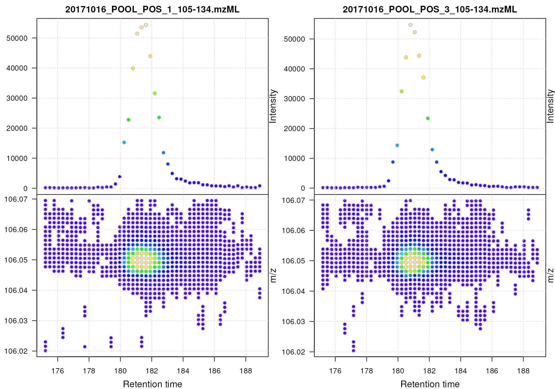
Profile data for Serine.
The lower panel of the plot shows all mass peaks measured by the instrument: each point represents one mass peak with its intensity being color coded (blue representing low, yellow high intensity). Each column of data points represents data from the same spectrum. The upper panel of the plot shows a chromatographic visualization of the data from the lower panel, i.e., for each retention time (spectrum) the sum of intensities within the m/z range is shown.
Note that, while it would be possible to create such a plot for the full MS data of an experiment, this type of visualization works best for small m/z - retention time regions.
Next, we smooth the data in each spectrum using a
Savitzky-Golay filter, which usually improves data quality by reducing
noise. Subsequently we perform the centroiding of the data based on a
simple peak-picking strategy that reports the maximum signal for each
mass peak in each spectrum. Finally, we replace the spectra in the data
(MsExperiment) object with the centroided spectra and
visualize the result repeating the visualization from above.
#' Smooth and centroid the spectra data
sps_cent <- spectra(mse) |>
    smooth(method = "SavitzkyGolay", halfWindowSize = 6L) |>
    pickPeaks(halfWindowSize = 2L)

#' Replace spectra in the original data object
spectra(mse) <- sps_cent

#' Plot the centroided data for Serine
mse |>
    filterRt(rt = c(175, 189)) |>
    filterMzRange(mz = c(106.02, 106.07)) |>
    plot()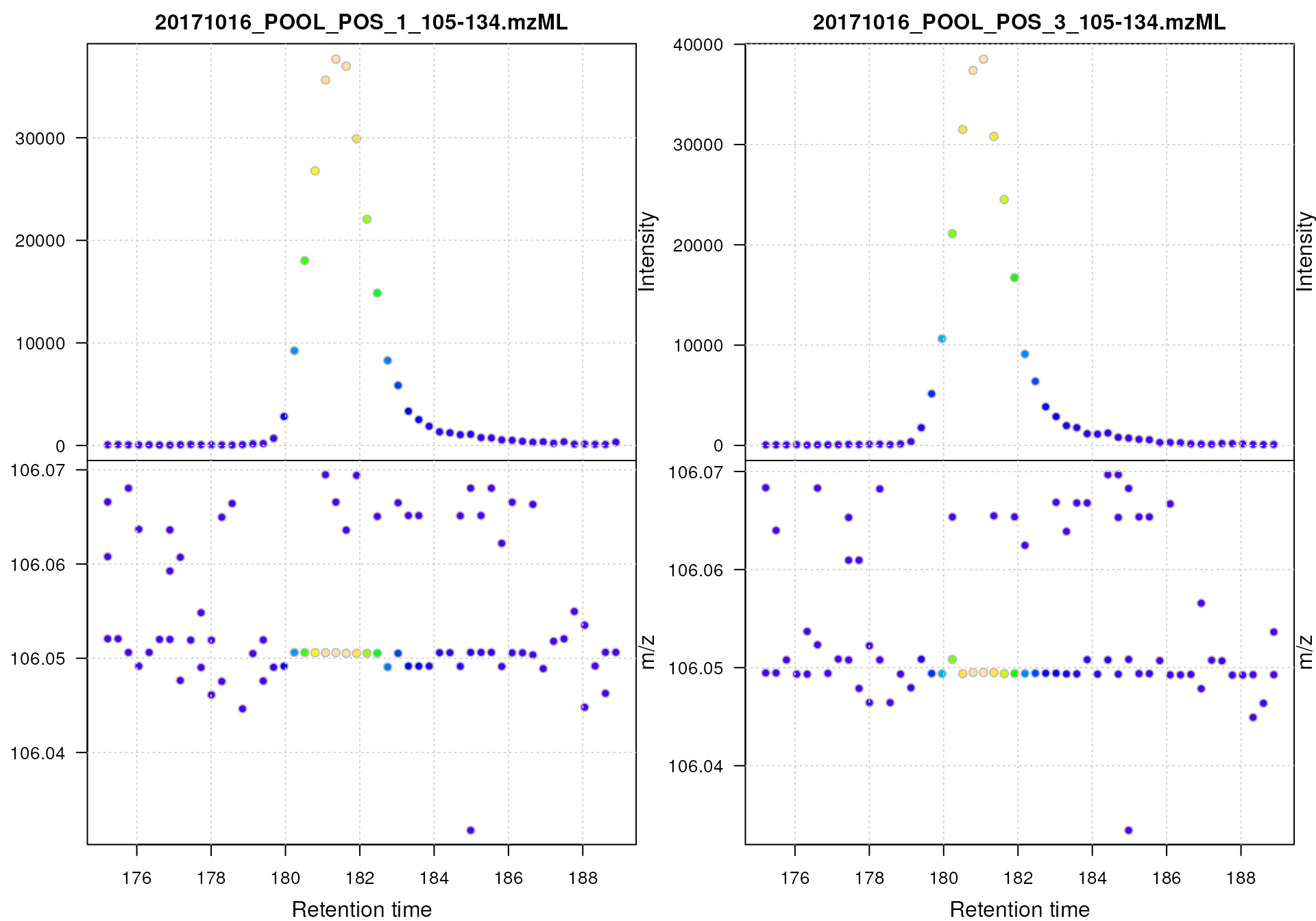
Centroided data for Serine.
The impact of the centroiding is clearly visible: each signal for an
ion in a spectrum was reduced to a single data point. For more advanced
centroiding options, that can also fine-tune the m/z value of
the reported centroid, see the documentation of the
pickPeaks() function or the centroiding vignette of the
MSnbase
package.
While we could now simply proceed with the data analysis, we below save the centroided MS data to mzML files to also illustrate how the Spectra package can be used to export MS data.
We use the export() function for data export of the
centroided Spectra object. Parameter backend
allows to specify the MS data backend that should be used for the
export, and that will also define the data format (use
backend = MsBackendMzR() to export data in mzML format).
Parameter file defines, for each spectrum, the name of the
file to which its data should be exported.
#' Export the centroided data to new mzML files.
export(spectra(mse), backend = MsBackendMzR(),
       file = basename(dataOrigin(spectra(mse))))
We can then import the centroided data again from the newly generated mzML files and proceed with the analysis.
#' Re-import the centroided data.
fls <- basename(fls)

#' Read the centroided data.
mse <- readMsExperiment(fls, sampleData = pd)
Thus, with few lines of R code we performed MS data centroiding in R which gives us possibly more, and better, control over the process and enable also (parallel) batch processing.
Preprocessing of LC-MS data
Preprocessing of (untargeted) LC-MS data aims at detecting and quantifying the signal from ions generated from all molecules present in a sample. It consists of the following 3 steps: chromatographic peak detection, retention time alignment and correspondence (also called peak grouping). The resulting matrix of feature abundances can then be used as an input in downstream analyses including data normalization, identification of features of interest and annotation of features to metabolites. In the following sections we perform such preprocessing of our test data set, adapting the settings for the preprocessing algorithms to our data.
Chromatographic peak detection
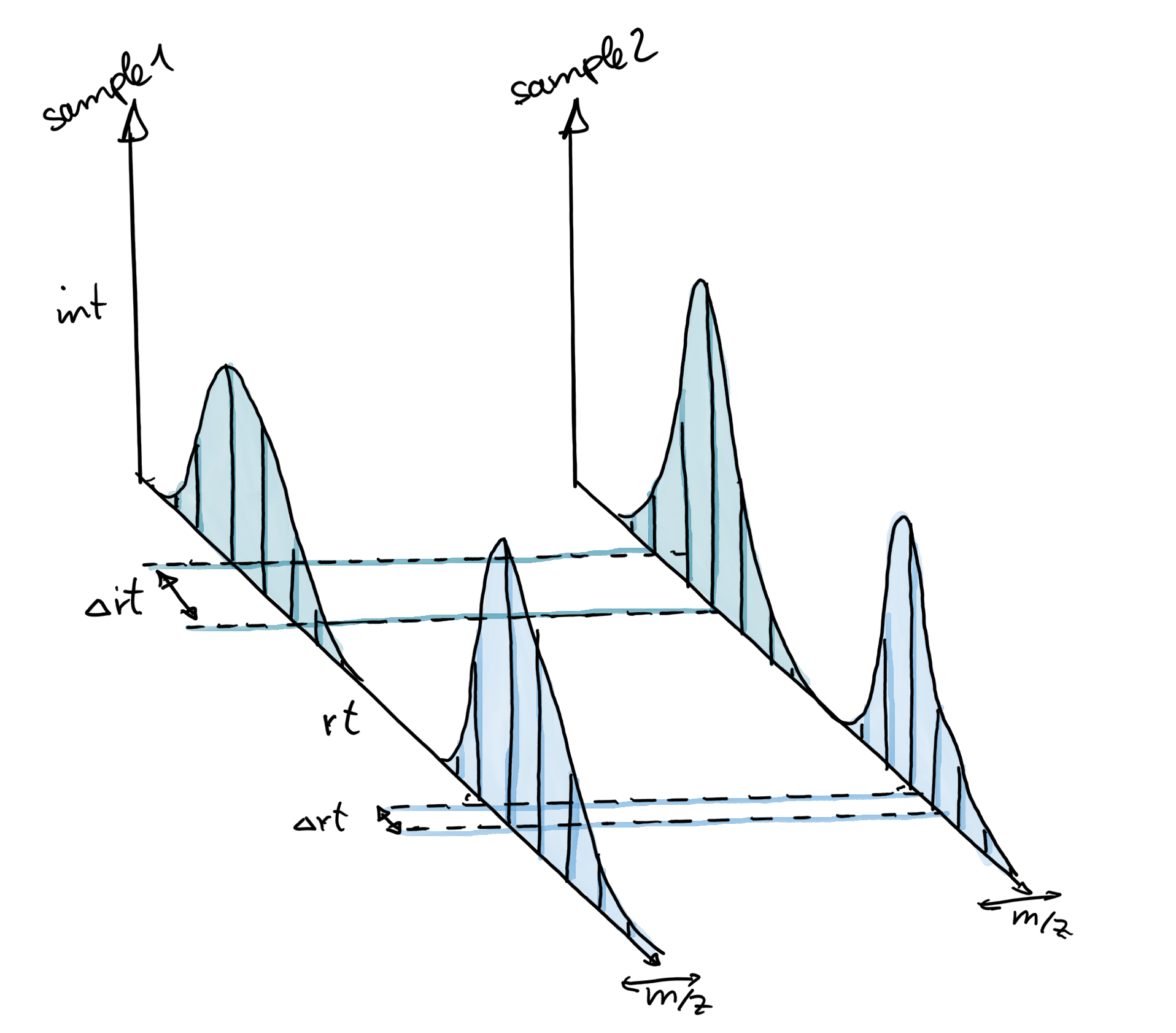
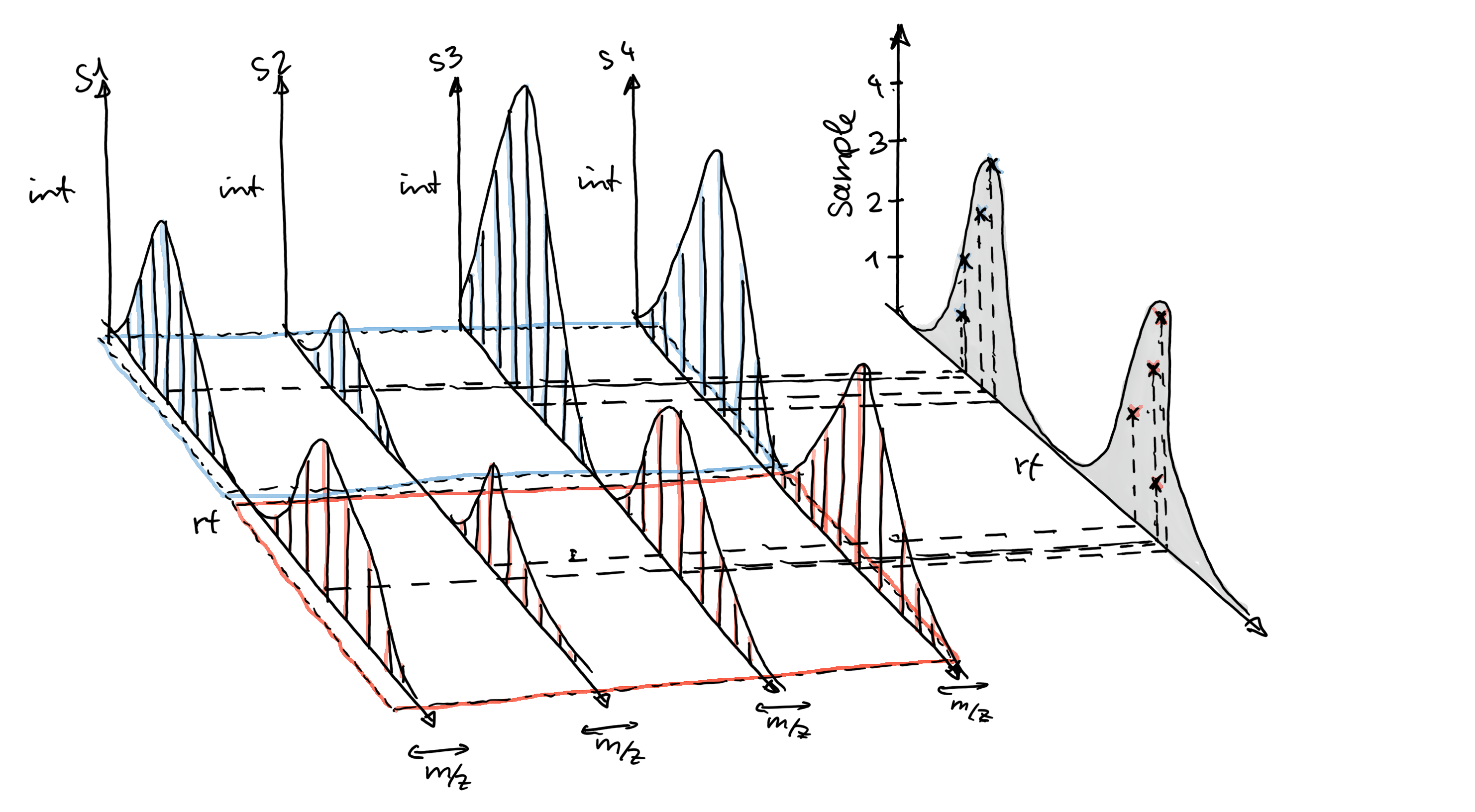
Chromatographic peak detection aims to identify peaks along the retention time axis that represent the signal from individual compounds’ ions. This involves identifying and quantifying such signals as shown in the sketch below.

Such peak detection can be performed with the xcms package
using its findChromPeaks() function. Several peak detection
algorithms are available that can be selected and configured with their
respective parameter objects:
-
MatchedFilterParamto perform peak detection as described in the original xcms article (Smith et al. 2006), -
CentWaveParamto perform a continuous wavelet transformation (CWT)-based peak detection (Tautenhahn et al. 2008) and -
MassifquantParamto perform a Kalman filter-based peak detection (Conley et al. 2014).
Additional peak detection algorithms for direct injection data are also available in xcms, but not discussed here.
In our example we use the centWave algorithm that performs
peak detection in two steps: first it identifies regions of
interest in the m/z - retention time space and
subsequently detects peaks in these regions using a continuous wavelet
transform (see the original publication (Tautenhahn et al. 2008) for more details). The
algorithm can be configured with several parameters (see
?CentWaveParam), with the most important being
peakwidth and ppm. peakwidth
defines the minimal and maximal expected width of the peak in retention
time dimension and depends thus on the setup of the employed LC-MS
system making this parameter highly data set dependent. ppm
on the other hand depends on the precision of the MS instrument. In this
section we describe how settings for these parameters can be empirically
determined for a data set.
Generally, it is strongly discouraged to blindly use the default parameters for any of the peak detection algorithms. To illustrate this we below extract the EIC for serine and run a centWave-based peak detection on that data using centWave’s default settings.
#' Get the EIC for serine in all files
serine_chr <- chromatogram(mse, rt = c(164, 200),
                           mz = serine_mz + c(-0.005, 0.005),
                           aggregationFun = "max")

#' Get default centWave parameters
cwp <- CentWaveParam()

#' "dry-run" peak detection on the EIC.
res <- findChromPeaks(serine_chr, param = cwp)
chromPeaks(res)
## mz mzmin mzmax rt rtmin rtmax into intb maxo sn row columnThe peak matrix returned by chromPeaks() is empty, thus,
with the default settings centWave failed to identify any
chromatographic peak in the EIC for serine. The default values for the
parameters are shown below:
#' Default centWave parameters
cwp
## Object of class: CentWaveParam
## Parameters:
## - ppm: [1] 25
## - peakwidth: [1] 20 50
## - snthresh: [1] 10
## - prefilter: [1] 3 100
## - mzCenterFun: [1] "wMean"
## - integrate: [1] 1
## - mzdiff: [1] -0.001
## - fitgauss: [1] FALSE
## - noise: [1] 0
## - verboseColumns: [1] FALSE
## - roiList: list()
## - firstBaselineCheck: [1] TRUE
## - roiScales: numeric(0)
## - extendLengthMSW: [1] FALSE
## - verboseBetaColumns: [1] FALSEParticularly the setting for peakwidth does not fit our
data. The default for this parameter expects chromatographic peaks
between 20 and 50 seconds wide. When we plot the extracted ion
chromatogram (EIC) for serine we can however see that these values are
way too large for our UHPLC-based data set (see below).
#' Plot the EIC
plot(serine_chr)
Extracted ion chromatogram for serine.
For serine, the chromatographic peak is about 5 seconds wide. We thus
adapt the peakwidth for the present data set and repeat the
peak detection using these settings. In general, the lower and upper
peak width should be set to include most of the expected chromatographic
peak widths. A good rule of thumb is to set it to about half to about
twice the average expected peak width. For the present data set we thus
set peakwidth = c(2, 10). In addition, by setting
integrate = 2, we select a different peak boundary
estimation algorithm. This works particularly well for non-gaussian peak
shapes and ensures that also signal from the peak’s tail is integrated
(eventually re-run the code with the default integrate = 1
to compare the two approaches).
#' Adapt centWave parameters
cwp <- CentWaveParam(peakwidth = c(2, 10), integrate = 2)

#' Run peak detection on the EIC
serine_chr <- findChromPeaks(serine_chr, param = cwp)

#' Plot the data and higlight identified peak area
plot(serine_chr)
EIC for Serine with detected chromatographic peak
Acceptable values for parameter peakwidth can thus be
derived through visual inspection of EICs for ions known to be present
in the sample (e.g. of internal standards). Ideally, this should be done
for several compounds/ions. Tip: ensure that the EIC contains
also enough signal left and right of the actual chromatographic peak to
allow centWave to properly estimate the background noise.
Alternatively, or in addition, reduce the value for the
snthresh parameter for peak detection performed on
EICs.
With our data set-specific peakwidth we were able to
detect the peak for serine (highlighted in grey in the plot above). We
can now use the chromPeaks() function to extract the
information on identified chromatographic peaks from our object.
#' Extract identified chromatographic peaks from the EIC
chromPeaks(serine_chr)
## mz mzmin mzmax rt rtmin rtmax into intb
## mzmin 106.0499 106.0449 106.0549 181.072 178.282 187.21 70373.61 70042.87
## maxo sn row column
## mzmin 38517.76 609 1 2The result is returned as a matrix with each row
representing one identified chromatographic peak. The retention time
ranges of the peaks are provided in columns "rtmin" and
"rtmax", the integrated peak area (i.e., the
abundance of the ion) in column "into", the
maximal signal of the peak in column "maxo" and the signal
to noise ratio in column"sn". With our adapted settings we
were thus able to identify a chromatographic peak for the serine ion in
each of the two samples.
The second important parameter for centWave is
ppm which is used in the initial definition of the
regions of interest (ROI) in which the actual peak detection is
then performed. To define these ROI, the algorithm evaluates for each
mass peak in a spectrum whether a mass peak with a similar m/z
(and a reasonably high intensity) is also found in the subsequent
spectrum. For this, only mass peaks with a difference in their
m/z smaller than ppm in consecutive scans are
considered. To illustrate this, we plot again the full MS data for the
data subset containing signal for serine.
#' Restrict to data containing signal from serine
srn <- mse |>
    filterRt(rt = c(179, 186)) |>
    filterMzRange(mz = c(106.04, 106.07))

#' Plot the data
plot(srn)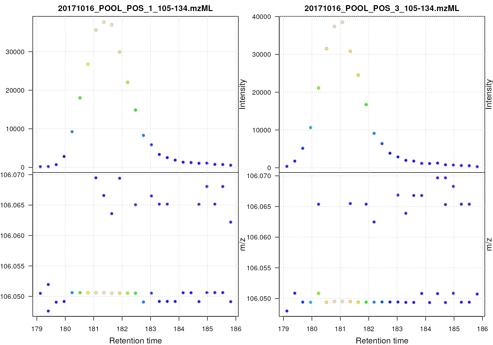
We can observe some scattering of the data points around an m/z of 105.05 in the lower panel of the above plot. This scattering also decreases with increasing signal intensity (as for many MS instruments the precision of the signal increases with the intensity). To quantify the observed differences in m/z values for the signal of serine we restrict the data to a bona fide region with signal for the serine ion. Below we first subset the data to the first file and then restrict the m/z range to values between 106.045 and 106.055.
#' Reduce the data set to signal of the [M+H]+ ion of serine
srn_1 <- srn[1] |>
    filterMzRange(c(106.045, 106.055)) |>
    spectra()
This restricted the MS data to spectra with a single mass peak per spectrum (presumably representing signal from the serine ion).
lengths(srn_1)## [1] 1 2 1 1 1 1 1 1 1 1 1 1 1 1 1 1 1 1 1 1 1 1 1 1 1We next extract the m/z values of the peaks from the consecutive scans and calculate the absolute difference between them.
#' Calculate the difference in m/z values between scans
mz_diff <- srn_1 |>
    mz() |>
    unlist() |>
    diff() |>
    abs()
mz_diff
## mz mz mz mz
## 2.904861e-03 4.357321e-03 2.904891e-03 1.179878e-04 1.452442e-03 0.000000e+00
## mz mz mz mz mz mz
## 1.684509e-05 0.000000e+00 0.000000e+00 7.233670e-05 0.000000e+00 0.000000e+00
## mz mz mz mz mz mz
## 7.624200e-07 1.452441e-03 1.452441e-03 1.358206e-03 0.000000e+00 0.000000e+00
## mz mz mz mz mz mz
## 1.425717e-03 0.000000e+00 1.452441e-03 1.480143e-03 0.000000e+00 0.000000e+00
## mz
## 1.493783e-03We can also express these differences in ppm (parts per million) of the average m/z of the peaks.
##                                     mz           mz           mz           mz
## 27.391410160 41.087396603 27.391691523  1.112566483 13.695817196  0.000000000
##           mz           mz           mz           mz           mz           mz
##  0.158840954  0.000000000  0.000000000  0.682099561  0.000000000  0.000000000
##           mz           mz           mz           mz           mz           mz
##  0.007189246 13.695808133 13.695808133 12.807212147  0.000000000  0.000000000
##           mz           mz           mz           mz           mz           mz
## 13.443812242  0.000000000 13.695807986 13.957023433  0.000000000  0.000000000
##           mz
## 14.085643094
The difference in m/z values for the serine data is thus
between 0 and 27 ppm. The maximum value could then be used for
centWave’s ppm parameter. Ideally, this should be evaluated
for several ions and could be set to a value that allows to capture the
full chromatographic peaks for most of the tested ions. Also, the value
for this parameter is generally much higher then the instrument
precision (for the present instrument that would have been 5 ppm). The
value should thus be set to a value that allows/accepts some
variance.
We can next perform the peak detection on the full data set using our
settings for the ppm and peakwidth
parameters.
#' Perform peak detection on the full data set
cwp <- CentWaveParam(peakwidth = c(2, 10), ppm = 30, integrate = 2)
mse <- findChromPeaks(mse, param = cwp)
The results form the chromatographic peak detection were added by the
findChromPeaks() to our mse variable which now
is an XcmsExperiment object that, by extending the
MsExperiment class inherits all of its functionality and
properties, but in addition contains also all xcms
preprocessing results.
mse## Object of class XcmsExperiment
## Spectra: MS1 (1862)
## Experiment data: 2 sample(s)
## Sample data links:
## - spectra: 2 sample(s) to 1862 element(s).
## xcms results:
## - chromatographic peaks: 644 in MS level(s): 1We can extract the results from the peak detection step (as above)
with the chromPeaks() function. The optional parameters
rt and mz would allow to extract peak
detection results for a specified m/z - retention time region.
In our example we extract all chromatographic peaks between an
m/z range from 106 to 108 and a retention time from 150 to
190.
#' Access the peak detection results from a specific m/z - rt area
chromPeaks(mse, mz = c(106, 108), rt = c(150, 190))
## mz mzmin mzmax rt rtmin rtmax into intb
## CP133 106.0625 106.0606 106.0636 173.264 171.869 174.380 516.3588 509.4463
## CP146 107.0653 107.0652 107.0653 173.543 171.032 179.682 11318.2801 11309.9091
## CP157 107.0532 107.0522 107.0537 181.356 179.682 183.309 2905.1158 2901.7678
## CP167 106.0506 106.0505 106.0506 181.356 178.845 187.773 74181.7823 73905.2115
## CP469 106.0633 106.0609 106.0652 172.701 170.748 174.654 559.5491 553.7921
## CP477 107.0656 107.0655 107.0657 172.980 169.632 178.003 11372.6845 11166.3372
## CP492 107.0538 107.0510 107.0540 181.072 178.840 183.304 3155.0100 3149.2053
## CP512 106.0496 106.0494 106.0508 181.072 178.282 187.210 70373.6099 70109.3562
## maxo sn sample
## CP133 426.6084 35 1
## CP146 4936.6783 4936 1
## CP157 1628.9510 186 1
## CP167 37664.9371 685 1
## CP469 381.6084 54 2
## CP477 4569.1399 79 2
## CP492 2297.7972 230 2
## CP512 38517.7622 830 2Again, each row in this matrix contains one identified
chromatographic peak with columns "mz",
"mzmin", "mzmax", "rt",
"rtmin" and "rtmax" defining it’s
position (and size) in the m/z - rt plane and
"into" and "maxo" its (integrated and maximum)
intensity. Column "sample" indicates in which of our
samples (data files) the peak was identified.
The chromatographic peak table above contains pairs of peaks with similar retention times and a difference in m/z values of about one. Together with the observed differences in intensities, this could indicate that one of the peaks represents the carbon 13 isotope and one the monoisotopic compound. This is frequently observed in untargeted metabolomics.
As a general overview of the peak detection results it can also be helpful to determine (and eventually) plot the number of identified chromatographic peaks per sample. Below we count the number of peaks per sample.
#' Count peaks per file
chromPeaks(mse)[, "sample"] |>
    table()
##
## 1 2
## 323 321About the same number of peaks was identified, which is to be expected since both files contain measurements from the same sample (the QC pool).
As an additional visual quality assessment, we can also plot the
location of the identified chromatographic peaks in the m/z -
retention time space for each data file using the
plotChromPeaks() function.
#' Plot the location of peaks in the m/z - rt plane
par(mfrow = c(1, 2))
plotChromPeaks(mse, 1)
plotChromPeaks(mse, 2)
Location of the identified chromatographic peaks in the m/z - rt space.
Again, similar pattern are expected to be present for the two data files.
After chromatographic peak detection it is generally a good idea to visually inspect individual chromatographic peaks and evaluate the performance of the peak detection step. This could be done by plotting EICs of known compounds/ions in the data or by randomly selecting chromatographic peaks. m/z - retention time regions for random peaks could be defined using the example code below.
#' Select 4 random peaks
npeaks <- nrow(chromPeaks(mse))
idx <- sample(seq_len(npeaks), 4)

#' Extract m/z-rt regions for 4 random peaks
mz_rt <- chromPeaks(mse)[idx, c("rtmin", "rtmax", "mzmin", "mzmax")]

#' Expand the rt range by 10 seconds on both sides
mz_rt[, "rtmin"] <- mz_rt[, "rtmin"] - 10
mz_rt[, "rtmax"] <- mz_rt[, "rtmax"] + 10
#' Expand the m/z range by 0.005 on both sides
mz_rt[, "mzmin"] <- mz_rt[, "mzmin"] - 0.005
mz_rt[, "mzmax"] <- mz_rt[, "mzmax"] + 0.005

#' Display the randomly selected regions
mz_rt
## rtmin rtmax mzmin mzmax
## CP110 141.781 167.919 118.0812 118.0915
## CP158 170.798 193.309 108.0477 108.0606
## CP064 64.217 88.960 117.0796 117.0912
## CP483 167.444 191.072 129.6296 129.6445For our example we however manually define m/z - retention
time regions (similarly as it could be done for known compounds). Below
we extract the EICs for these regions with the
chromatogram() function and subsequently plot them.
Identified chromatographic peaks within the plotted regions will by
default be highlighted in a semitransparent grey color.
#' Define m/z - retention time regions for EICs
mz_rt <- rbind(c(106.045, 106.055, 165, 195),
               c(132.096, 132.107, 135, 160),
               c(125.981, 125.991, 195, 215),
               c(105.468, 105.478, 190, 215))

#' Extract the EICs
eics <- chromatogram(mse, mz = mz_rt[, 1:2], rt = mz_rt[, 3:4], )
#' Plot the EICs
plot(eics)
While the peak detection worked nicely for the signals in the upper
row, it failed to define chromatographic peaks containing the full
signal in the lower row. In both cases, the signal was split into
separate chromatographic peaks within the same sample. This is a common
problem with centWave on such noisy and broad signals. We could
either try to adapt the centWave settings and repeat the
chromatographic peak detection or use the
refineChromPeaks() function that allows to post-process
peak detection results and fix such problems (see also the documentation
of the refineChromPeaks() function for all possible
refinement options).
To fuse the wrongly split peaks in the second row, we use the
MergeNeighboringPeaksParam algorithm that merges
chromatographic peaks that are overlapping on the m/z and
retention time dimension for which the signal between them is higher
than a certain value. We specify expandRt = 4 to expand the
retention time width of each peak by 4 seconds on each side and set
minProp = 0.75. All chromatographic peaks with a distance
tail-to-head in retention time dimension that is less than
2 * expandRt and for which the intensity between them is
higher than 75% of the lower (apex) intensity of the two peaks are thus
merged. We below apply these settings on the EICs and evaluate the
result of this post-processing.
#' Define the setting for the peak refinement
mpp <- MergeNeighboringPeaksParam(expandRt = 4, minProp = 0.75)

#' Perform the peak refinement on the EICs
eics <- refineChromPeaks(eics, param = mpp)

#' Plot the result
plot(eics)
The peak post-processing was able to merge the signal for the neighboring peaks in the lower panel, while keeping the peaks for the different isomers present in the top right plot separate. We next apply this same peak refinement on the full data set.
#' Perform peak refinement on the full data set
mse <- refineChromPeaks(mse, param = mpp)
The number of peaks per sample after peak refinement is shown below.
chromPeaks(mse)[, "sample"] |>
    table()
##
## 1 2
## 297 292Also, refineChromPeaks() adds information on the peak
refinement to the object’s chromPeakData() data frame which
provides additional metadata information for each chromatographic
peak:
chromPeakData(mse)## DataFrame with 589 rows and 3 columns
## ms_level is_filled merged
## <integer> <logical> <logical>
## CP001 1 FALSE FALSE
## CP002 1 FALSE FALSE
## CP003 1 FALSE FALSE
## CP004 1 FALSE FALSE
## CP005 1 FALSE FALSE
## ... ... ... ...
## CP669 1 FALSE TRUE
## CP670 1 FALSE TRUE
## CP671 1 FALSE TRUE
## CP672 1 FALSE TRUE
## CP673 1 FALSE TRUEAnd the number of merged peaks is thus:
sum(chromPeakData(mse)$merged)## [1] 29Retention time alignment
While chromatography helps to better discriminate between analytes it
is also affected by variances that lead to shifts in retention times
between measurement runs. Such differences can usually already be seen
in a base peak chromatogram or total ion chromatogram. We thus extract
and plot below the BPC for our data set. In the
chromatogram() call, we set the optional parameter
chromPeaks = "none" to avoid the additional extraction of
all identified chromatographic peaks.
#' Extract base peak chromatograms
bpc_raw <- chromatogram(mse, aggregationFun = "max", chromPeaks = "none")
plot(bpc_raw, peakType = "none")
BPC of all files.
Both samples were measured with the same setup in the same measurement run, but still small drifts of the signal are visible. These were also already visible in the EIC for serine, that we plot again below.

For the serine signal, there seems to be a retention time shift of about 1 second between the two samples. The alignment step aims to minimize these retention time differences between all samples within an experiment (see below for an illustration).
In xcms, the alignment can be performed with the
adjustRtime() function and one of the available alignment
algorithms, that can be selected, and configured, with the respective
parameter objects:
PeakGroupsParam: the peakGroups (Louail et al. 2025) method aligns samples based on the retention times of a set of so called anchor peaks (or housekeeping peaks) in the different samples of an experiment. These peaks are supposed to represent signal from ions expected to be present in most of the samples of an experiment and the method aligns these samples by minimizing the between-sample retention time differences observed for these peaks.ObiwarpParam: obiwarp (Prince and Marcotte 2006) performs retention time adjustment based on the full m/z - retention time data. See the documentation forObiwarpParamor the xcms vignette for more information.
While, by default, retention time shifts are estimated on the full data set, it would also be possible to estimate them on a subset of samples, such as repeatedly measured QC samples (e.g. sample pools) and adjust the full experiment based on these. See the alignment section in the xcms vignette for more information on this subset-based alignment. Note that such a subset-based alignment requires the samples to be organized in the order in which they were measured. Also, recently, functionality was added to xcms to perform the alignment on pre-selected signals (e.g. retention times of internal standards) or to align a data set against an external reference.
For our example we use the peakGroups method that, as
mentioned above, aligns samples based on the retention times of
anchor peaks. To define these, we need to first run an initial
correspondence analysis and group chromatographic peaks across samples.
Below we use the peakDensity method for correspondence (details
about this method and explanations on the choices of its parameters are
provided in the next section). In brief, parameter
sampleGroups defines to which sample group of the
experiment individual samples belong to, and parameter
minFraction specifies the proportion of samples (of one of
the sample groups defined in sampleGroups) in which a
chromatographic peak needs to be detected to group them into an LC-MS
feature. Chromatographic peaks will be grouped to features if their
difference in m/z and retention times is below the defined
thresholds and if in at least minFraction * 100 percent of
samples of at least one sample group a chromatographic peak was
detected. For our example we use the sample group definition in the
sampleData of our mse variable and set
minFraction = 1 requiring thus a chromatographic peak to be
identified in all (100%) of available samples to define a feature.
Generally, if correspondence is performed on more heterogeneous samples,
minFraction values between 0.6 and 0.8 could be used
instead. Since the aim of this initial correspondence is to define some
(presumably well separated) groups of chromatographic peaks across the
samples, its settings does not need to be fully optimized.
#' Define the settings for the initial peak grouping - details for
#' choices in the next section.
pdp <- PeakDensityParam(sampleGroups = sampleData(mse)$group, bw = 1.8,
                        minFraction = 1, binSize = 0.01, ppm = 10)
mse <- groupChromPeaks(mse, pdp)
This step now grouped chromatographic peaks across samples and
defined so called LC-MS features (or simply features). We can thus now
run the alignment using the peakGroups algorithm that aligns
the data by minimizing differences in retention times of anchor
peaks (i.e. selected features with chromatographic peaks detected
in most samples). The main parameter to define these anchor peaks is
minFraction. Similar to the definition above,
minFraction refers to the proportion of samples in which a
chromatographic peak needs to be present, only, here we don’t consider
the different sample groups, but the whole data set. By setting
minFraction = 1 we base the alignment on features with
peaks identified in 100% of the samples in the data set. For alignments
that are based on repeatedly measured samples (e.g. also for
subset-based alignment on sample pools) values >= 0.9
can be used. Otherwise, values between 0.7 and 0.9 might be more
advisable to ensure that a reasonable set of features are selected.
To evaluate anchor peaks that would be selected based on the defined
settings, we can also use the adjustRtimePeakGroups()
method:
#' Get the anchor peaks that would be selected
pgm <- adjustRtimePeakGroups(mse, PeakGroupsParam(minFraction = 1))
head(pgm)
## 20171016_POOL_POS_1_105-134.mzML 20171016_POOL_POS_3_105-134.mzML
## FT136 22.601 24.270
## FT163 25.391 25.665
## FT030 25.670 25.665
## FT212 26.507 26.502
## FT056 26.786 27.060
## FT162 28.739 28.734Ideally, if possible, the anchor peaks should span most of the retention time range to allow alignment of the full LC runs. Below evaluate the distribution of retention times of the anchor peaks in the first sample.
#' Evaluate distribution of anchor peaks' rt in the first sample
quantile(pgm[, 1])
## 0% 25% 50% 75% 100%
## 22.601 155.408 180.240 194.190 259.478Anchor peaks cover thus most of the retention time range.
After having identified the features that should be used as anchor
peaks (based on the minFraction parameter) the algorithm
minimizes the observed between-sample retention time differences for
these. Parameter span defines the degree of smoothing of
the loess function that is used to allow different regions along the
retention time axis to be adjusted by a different factor. A value close
to 0 will most likely cause overfitting, while a value of 1 would cause
all retention times of a sample to be shifted by a constant value.
Values between 0.4 and 0.6 seem to be reasonable for most
experiments.
#' Define settings for the alignment
pgp <- PeakGroupsParam(minFraction = 1, span = 0.6)
mse <- adjustRtime(mse, param = pgp)
After an alignment it is suggested to evaluate its results using the
plotAdjustedRtime() function. This function plots the
differences between adjusted and raw retention times for each sample on
the y-axis along the adjusted retention times on the x-axis (each line
hence representing the retention time adjustment of one sample/file).
Points indicate the position of individual hook peaks along the
retention time axis, with a dotted line connecting the peaks belonging
to the same feature (for which the algorithm minimized the difference in
retention times).
#' Plot the difference between raw and adjusted retention times
plotAdjustedRtime(mse)
grid()
Alignment results: differences between raw and adjusted retention times for each sample.
As a rule of thumb, the differences between raw and adjusted retention times in the plot above should be reasonable. Also, if possible, anchor peaks (indicated with black points in the plot above) should be present along a wide span of the retention time range, to avoid the need for extrapolation (which usually results in a too strong adjustment). For our example, the largest adjustments are between 1 and 2 seconds, which is reasonable given that the two samples were measured during the same measurement run. Also, features used for the alignment (i.e. anchor peaks) are spread across the full retention time range.
To evaluate the impact of the alignment we next also plot the BPC
before and after alignment. In a similar way as before, we set
chromPeaks = "none" in the chromatogram() call
to tell the function to not include any identified
chromatographic peaks in the returned chromatographic data.
par(mfrow = c(2, 1))

#' Plot the raw base peak chromatogram
plot(bpc_raw)
grid()

#' Plot the BPC after alignment
chromatogram(mse, aggregationFun = "max", chromPeaks = "none") |>
    plot()
grid()
BPC before (top) and after (bottom) alignment.
The base peak chromatograms are nicely aligned after retention time adjustment. In addition to this general assessment, the alignment result should also be evaluated for selected compounds (or internal standards). We thus below plot the EIC for the [M+H]+ ion for serine before and after alignment.
par(mfrow = c(1, 2), mar = c(4, 4.5, 1, 0.5))

#' EIC before alignment
plot(serine_chr)
grid()
#' EIC after alignment
serine_chr_adj <- chromatogram(mse, rt = c(164, 200),
                               mz = serine_mz + c(-0.01, 0.01),
                               aggregationFun = "max")
plot(serine_chr_adj)
grid()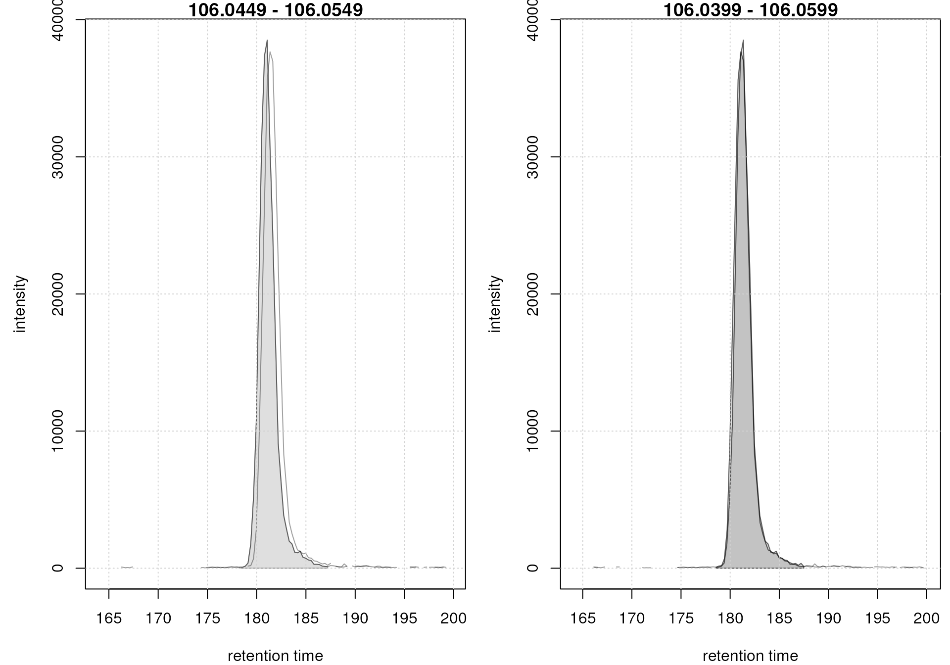
EIC for Serine before (left) and after (right) alignment
The serine peaks are also nicely aligned after retention time adjustment. Again, it is advisable to evaluate the impact of the alignment on several EICs, ideally also spread along the retention time range.
Note that adjustRtime(), in addition to the retention
times of the individual (MS1) spectra of all files, adjusted also the
retention times of the identified chromatographic peaks, as well as
retention times of possibly present MS2 spectra. The adjusted retention
times are stored as a new spectra variable "rtime_adjusted"
in the result object’s Spectra. The rtime()
function on the result object will by default return these (adjusted)
values.
Correspondence
The final step of the LC-MS preprocessing with xcms is the correspondence analysis, in which chromatographic peaks from the same types of ions (compounds) are grouped across samples to form the so called LC-MS features.
In xcms, correspondence is performed using the
groupChromPeaks() function. The correspondence algorithm
can be selected and configured with the respective parameter
objects:
NearestPeaksParam: performs peak grouping based on the proximity of chromatographic peaks from different samples in the m/z - retention time space, similar to the original correspondence method of mzMine (Katajamaa et al. 2006).PeakDensityParam: performs a simple and fast correspondence analysis based on the density of chromatographic peaks (from different samples) along the retention time axis within slices of small m/z ranges (Louail et al. 2025).
Both methods group chromatographic peaks from different samples with
similar m/z and retention times into features. For our example
we use the peak density method. This algorithm iterates through
small slices along the m/z dimension and groups, within each
slice, chromatographic peaks with similar retention times. The grouping
depends on the distribution (density) of chromatographic peaks from all
samples along the retention time axis. Peaks with similar retention time
will result in a higher peak density at a certain retention time and are
thus grouped together. The grouping depends on the smoothness
of the density curve and can be configured with parameter
bw.
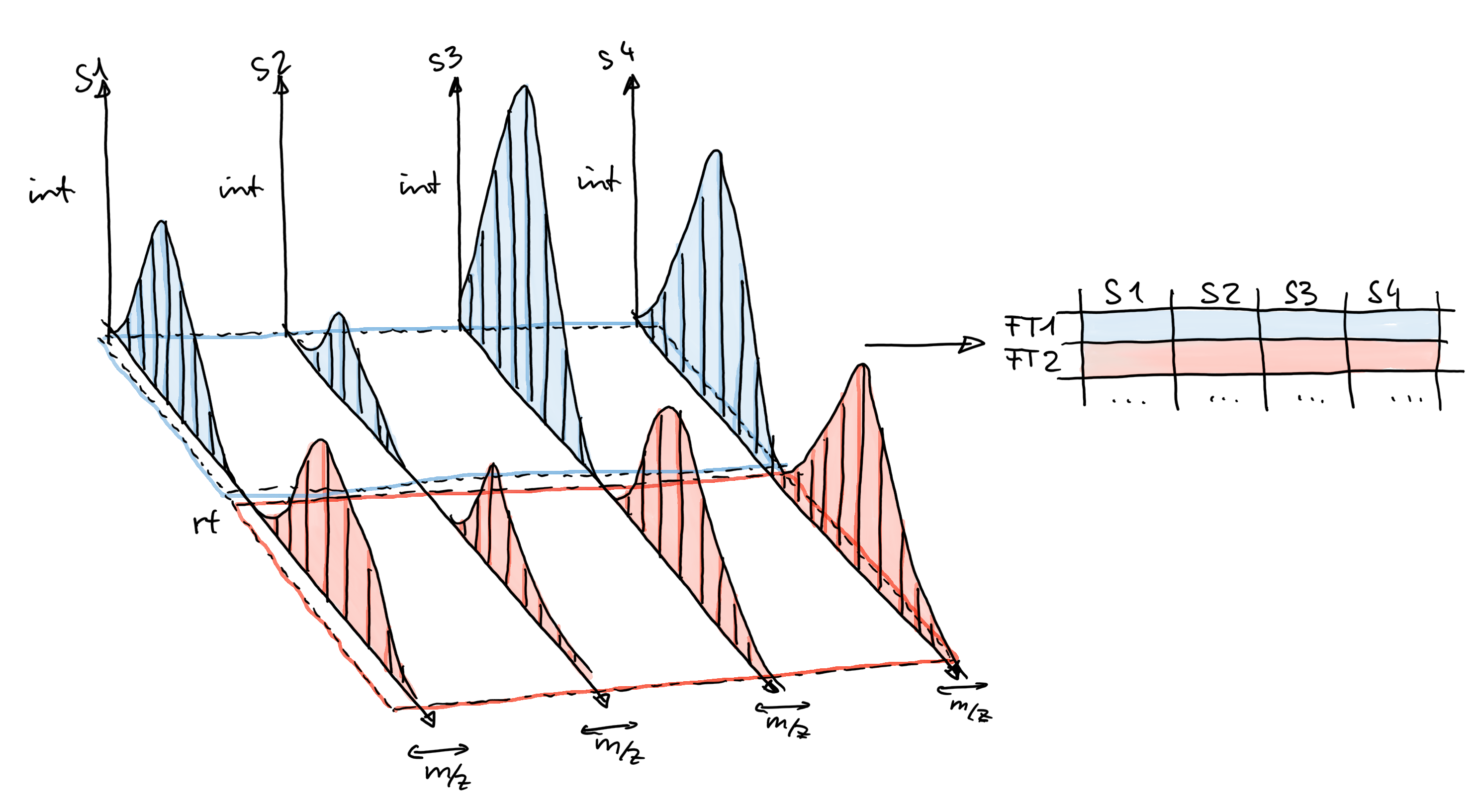
An illustration showing how chromatographic peaks within a small m/z range are grouped by the peakDensity method is shown in the sketch below.
Settings for this algorithm can be best tested and optimized using
the plotChromPeakDensity() function on extracted
chromatograms. We below extract a chromatogram for a m/z slice
containing signal for a [M+H]+ ion of serine and evaluate the
result from a peakDensity correspondence analysis using that
function. We use the default settings (bw = 30) and use
again the sample group assignment defined in
sampleData().
#' Extract a chromatogram for a m/z range containing serine
chr_1 <- chromatogram(mse, mz = serine_mz + c(-0.005, 0.005))

#' Default parameters for peak density; bw = 30
pdp <- PeakDensityParam(sampleGroups = sampleData(mse)$group, bw = 30)

#' Test these settings on the extracted slice
plotChromPeakDensity(chr_1, param = pdp)
The upper panel in the plot shows the chromatographic data for the
selected m/z slice with the identified peaks highlighted in
grey. The lower panel plots the retention time of identified
chromatographic peaks on the x-axis against the index of the sample in
which the peak was identified. Each chromatographic peak is thus
represented with a point in that plot (x-axis value being its retention
time and the y-axis value the sample in which it was identified). In our
example there was one chromatographic peak identified in each sample at
a retention time of about 180 seconds and these two peaks are thus
shown. The black solid line represents the density estimation
(i.e. distribution or retention times) of the identified chromatographic
peaks along the retention time axis. The smoothness of this curve (which
is created with the base R density() function) is
configured with the parameter bw. The peakDensity
algorithm assigns all chromatographic peaks within the same
peak of this density estimation curve to the same feature.
Chromatographic peaks assigned to the same feature are indicated with a
grey rectangle in the lower panel of the plot. In the present example,
because retention times of the two chromatographic peaks are very
similar, this rectangle is very narrow and looks thus more like a
vertical line. Based on this result, the default settings
(bw = 30) seemed to correctly define features. It is
however advisable to evaluate settings on multiple slices, ideally with
signal from more than one compound being present. Such slices could be
identified in e.g. a plot created with the plotChromPeaks()
function (see example in the chromatographic peak detection
section).
In our example we extract a chromatogram for an m/z slice containing signal for known isomers betaine and valine ([M+H]+ m/z 118.08625).
#' Plot the chromatogram for an m/z slice containing betaine and valine
mzr <- 118.08625 + c(-0.005, 0.005)
chr_2 <- chromatogram(mse, mz = mzr, aggregationFun = "max")

#' Correspondence in that slice using default settings
plotChromPeakDensity(chr_2, param = pdp)
Correspondence analysis with default settings on an m/z slice containing signal from multiple ions.
This slice contains signal from several ions resulting in multiple
chromatographic peaks along the retention time axis. With the default
settings, in particular with bw = 30, all these peaks were
however assigned to the same feature (indicated with the grey
rectangle). Signal from different ions would thus be treated as a single
entity. We repeat the analysis below with a strongly reduced value for
parameter bw.
#' Reducing the bandwidth
pdp <- PeakDensityParam(sampleGroups = sampleData(mse)$group, bw = 1.8)
plotChromPeakDensity(chr_2, param = pdp)
Correspondence analysis with reduced bw setting on a m/z slice containing signal from multiple ions.
Setting bw = 1.8 strongly reduced the smoothness of the
density curve resulting in a higher number of density peaks and
hence a nice grouping of (aligned) chromatographic peaks into separate
features. Note that the height of the peaks of the density curve are not
relevant for the grouping.
By having defined a bw appropriate for our data set, we
proceed and perform the correspondence analysis on the full data set.
Other parameters of peakDensity are binSize and
minFraction. The minFraction parameter
(already discussed above) defines the proportion of samples within at
least one sample group in which chromatographic peaks need to be
identified in order to define a feature.
binSize defines the m/z widths of the slices
along the m/z dimension the algorithm will iterate through.
This parameter thus translates into the maximal acceptable difference in
m/z values for peaks to be considered representing signal from
the same ion. The value depends on the resolution (and noise) of the
instrument, and should not be set to a too small value, but also not too
large (to avoid peaks from different ions, with slightly different
m/z but similar retention times, to be grouped into the same
feature). Note that by default a constant m/z
width is used, which might however not reflect the
m/z-dependent measurement error of some instruments (such as
TOF instruments). To address this, the parameter ppm was
recently added that allows to generate m/z-dependent bin sizes:
the width of the m/z slices increases by ppm of
the bin’s m/z along the m/z axis.
For our correspondence analysis we set the maximal acceptable
difference of chrom peaks’ m/z values with
binSize = 0.01 and ppm = 10, hence grouping
chromatographic peaks with similar retention time and with a difference
of their m/z values that is smaller than 0.01 + 10 ppm of their
m/z values. By setting minFraction = 0.4 we in
addition require for a feature that a chromatographic peak was detected
in >= 40% of samples of at least one sample group.
#' Set in addition parameter ppm to a value of 10
pdp <- PeakDensityParam(sampleGroups = sampleData(mse)$group, bw = 1.8,
                        minFraction = 0.4, binSize = 0.01, ppm = 10)

#' Perform the correspondence analysis on the full data
mse <- groupChromPeaks(mse, param = pdp)
mse
## Object of class XcmsExperiment
## Spectra: MS1 (1862)
## Experiment data: 2 sample(s)
## Sample data links:
## - spectra: 2 sample(s) to 1862 element(s).
## xcms results:
## - chromatographic peaks: 589 in MS level(s): 1
## - adjusted retention times
## - correspondence results: 357 features in MS level(s): 1The present data set is restricted to a quite narrow m/z
range, thus, the parameter ppm does not have a strong
impact. For real data sets, this parameter results in an
m/z-dependent m/z width of detected features. For
binSize = 0.01 and ppm = 10 and a data set
with an m/z range from 0 to 1000, the width of the m/z
bins would linearly increase, along the m/z axis, from an
initial size of 0.01 up to a value of 0.02 (the static size of 0.01 plus
10 ppm of the maximal m/z of 1000 which results in the maximal
bin size of 0.02). See also this
github issue for an example and discussion.
Over 300 features were identified in our example data set. Again, it
is suggested to evaluate the results on selected compounds/ions. We
therefore extract below the chromatogram for the m/z range
containing signals for betaine and valine. After a correspondence
analysis also feature definitions are extracted by the
chromatogram() call and we can show the results from the
actual correspondence analysis (based also on the settings that were
used) by setting simulate = FALSE in the
plotChromPeakDensity() call.
#' Extract chromatogram including signal for betaine and valine
chr_2 <- chromatogram(mse, mz = 118.08625 + c(-0.005, 0.005),
                      aggregationFun = "max")
#' Setting simulate = FALSE to show the actual correspondence results
plotChromPeakDensity(chr_2, simulate = FALSE)
Result of correspondence on an m/z slice containing the isomers valine and betaine.
We evaluate the results also on a different slice containing signal for ions from isomers leucine and isoleucine ([M+H]+ m/z 132.10191).
#' Extract chromatogram with signal for isomers leucine and isoleucine
chr_3 <- chromatogram(mse, mz = 132.10191 + c(-0.005, 0.005),
                      aggregationFun = "max")
plotChromPeakDensity(chr_3, simulate = FALSE)
Result of correspondence on an m/z slice containing the isomers leucine and isoleucine.
Despite being very close, chromatographic peaks of the two isomers were successfully grouped into separate features. Even the partially overlapping signal from a third ion eluting at about the same time and hence partially overlapping with the peak at a retention time of 152 seconds was grouped into its own, separate, feature. It is at the discretion of the data analysts to define how fine or coarse the feature grouping should be. Especially for larger experiments, with more samples and also larger variation in retention time it might not always be possible to completely separate all closely eluting ions from each other and sometimes it might be acceptable to group them into a single feature (keeping in mind that this feature would then however potentially represent signal from multiple different ions/compounds).
Similar to the peak detection and alignment results, also the results
from the correspondence analysis were added to the
XcmsExperiment object. These can be extracted with the
featureDefinitions() function, that extracts the
definition of the LC-MS features and the
featureValues() function that extracts the numerical matrix
with the feature abundances (in all samples). Below we extract the
definition of the features and display the first 6 rows.
#' Definition of the features
featureDefinitions(mse) |>
    head()
## mzmed mzmin mzmax rtmed rtmin rtmax npeaks POOL
## FT001 105.0418 105.0417 105.0418 167.68958 167.50191 167.87725 2 2
## FT002 105.0415 105.0415 105.0415 157.72336 157.72336 157.72336 1 1
## FT003 105.0697 105.0691 105.0703 31.80810 31.67412 31.94208 2 2
## FT004 105.1103 105.1100 105.1105 63.75036 63.45657 64.04414 2 2
## FT005 105.4734 105.4732 105.4736 201.57632 201.37059 201.78204 2 2
## FT006 105.7166 105.7160 105.7172 181.21537 181.08482 181.34592 2 2
## peakidx ms_level
## FT001 115, 393 1
## FT002 114 1
## FT003 21, 317 1
## FT004 49, 348 1
## FT005 261, 573 1
## FT006 138, 440 1Each row defines one feature and provides information on it’s
m/z (column "mzmed") and retention time (column
"rtmed"). The -min and -max columns list
the minimum and maximum rt or m/z value of the chromatographic
peaks assigned to the feature. Additional columns list the number of
chromatographic peaks that were assigned to the feature and the MS
level. Column "peakidx" provides the indices of the
chromatographic peaks in the chromPeaks() matrix that were
assigned to the feature - but generally users will not need or extract
that information.
The feature abundance matrix, which is the final result of the
xcms preprocessing, can be extracted with the
featureValues() function. By default, with parameter
method = "maxint", it returns for each feature the
integrated peak signal of the chromatographic peak with the highest
signal per sample. Note that this has only an effect for features with
more than one chromatographic peak per sample (i.e., if multiple
chromatographic peaks in the same sample were grouped
into the feature because of their closeness in retention time and
m/z value). Setting method = "sum" would in
contrast sum the abundances of such chromatographic peaks. Note that
method = "sum" is only suggested if, like in our example,
neighboring and overlapping peaks per sample were merged to avoid an
overestimation of the feature abundance. Below we extract the feature
abundances and show the first 6 rows.
#' Get abundances for the first 6 features
featureValues(mse, method = "sum") |>
    head()
## 20171016_POOL_POS_1_105-134.mzML 20171016_POOL_POS_3_105-134.mzML
## FT001 3202.7445 2285.2830
## FT002 3605.3915 NA
## FT003 744.8752 1057.4312
## FT004 18126.4603 19369.4039
## FT005 23243.6129 31960.3709
## FT006 671.5842 617.7545We could now use this feature matrix for any downstream analysis. Such feature matrix might however, as can also be seen in the second row above (feature FT002), contain missing values. These represent features for which no chromatographic peak was identified in one (or more) sample(s). While a number of imputation methods exist to deal with missing values, it might be more advisable to instead rescue signal. xcms provides such gap filling which is explained in the next section.
Gap filling
Missing values in feature matrices from an xcms-based preprocessing represent cases in which, in a particular sample, no chromatographic peak was identified in the m/z - retention time region of the feature. This could either represent a truly missing value (because the ion/compound was not present in that sample) or a failure of the peak detection algorithm to identify a peak (either because the measured signal was too noisy, or too low, or a combination of both).
To illustrate this we below define m/z - retention time regions containing signal of features with missing values, extract their EICs and plot them (using a different color for each sample). Note: these regions were identified by first visually inspecting EICs for all features with at least one missing value.
#' Define m/z - rt regions for selected examples with missing peaks
mz_rt <- rbind(c(109.661, 109.664, 192, 200),
               c(109.993, 109.998, 200, 215),
               c(125.586, 125.591, 195, 215),
               c(130.959, 130.961, 197, 201))

#' Extract their EICs and plot them
chrs <- chromatogram(mse, mz = mz_rt[, 1:2], rt = mz_rt[, 3:4])
plot(chrs, col = c("red", "blue"), lwd = 2)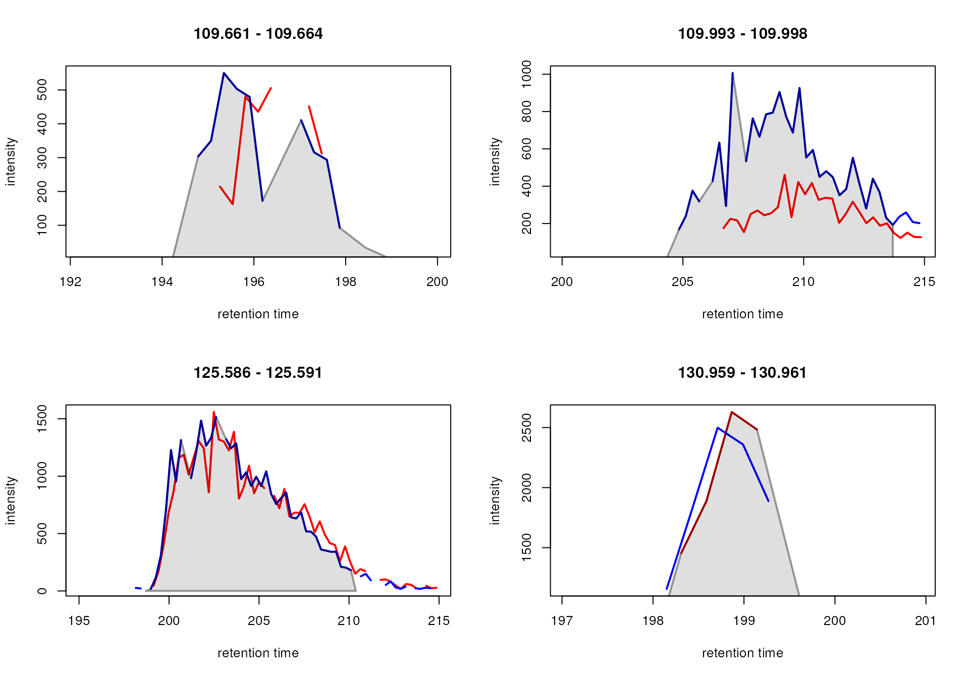
Examples of features for which a peak was only identified in one sample.
Indeed, for all these feature, chromatographic peak detection failed to identify a peak in one of the two samples (detected chromatographic peaks are indicated with a grey background color in the plot above). For the features in the upper panel, the signal was most likely too low, while for the bottom left feature the signal was likely too noisy, and for the bottom right too sparse (i.e. to few data points to properly detect a peak). In all cases, however, signal from (presumably) the same ion was measured in both samples. Thus, reporting a missing value would not be correct for these.
The aim of the gap filling is now to rescue signal
for such features by integrating the intensities measured within the
feature’s m/z - retention time area in the sample(s) in which
no chromatographic peak was detected. In xcms this can be done
with the fillChromPeaks() function and the
ChromPeakAreaParam parameter to configure the gap filling.
Below we perform gap filling showing also the number of missing values
before and after running fillChromPeaks().
#' Number of missing values
sum(is.na(featureValues(mse)))
## [1] 133
#' Perform gap filling
mse <- fillChromPeaks(mse, param = ChromPeakAreaParam())

#' Number of missing values after gap filling
sum(is.na(featureValues(mse)))
## [1] 25With fillChromPeaks() we could thus rescue
signal for all but 26 features. Also for the 4 example features from
above a signal was filled-in. Below we visualize the gap-filled
chromatographic peaks for these.
#' Extract their EICs and plot them
chrs <- chromatogram(mse, mz = mz_rt[, 1:2], rt = mz_rt[, 3:4])
plot(chrs, col = c("red", "blue"), lwd = 2)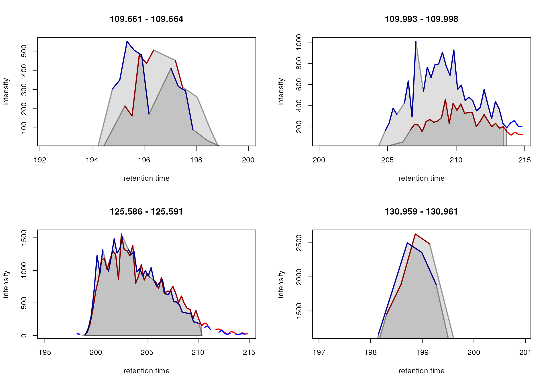
Features with filled-in signal.
In contrast, we identify and plot the EICs for features for which no signal could be filled-in (i.e. which still have missing values in one of the two samples).
#' Identify rows (features) with at least one missing value across samples
any_na <- featureValues(mse) |>
    rowSums() |>
    is.na()
#' Get the feature IDs for these
fts <- rownames(featureValues(mse))[any_na]

#' Extract the m/z - rt regions for these features
mz_rt <- featureArea(mse, features = fts)

#' Expand the retention time by 1 second on both sides
mz_rt[, "rtmin"] <- mz_rt[, "rtmin"] - 1
mz_rt[, "rtmax"] <- mz_rt[, "rtmax"] + 1

chrs_na <- chromatogram(mse, mz = mz_rt[, c("mzmin", "mzmax")],
                        rt = mz_rt[, c("rtmin", "rtmax")])

plot(chrs_na, col = c("red", "blue"), lwd = 2)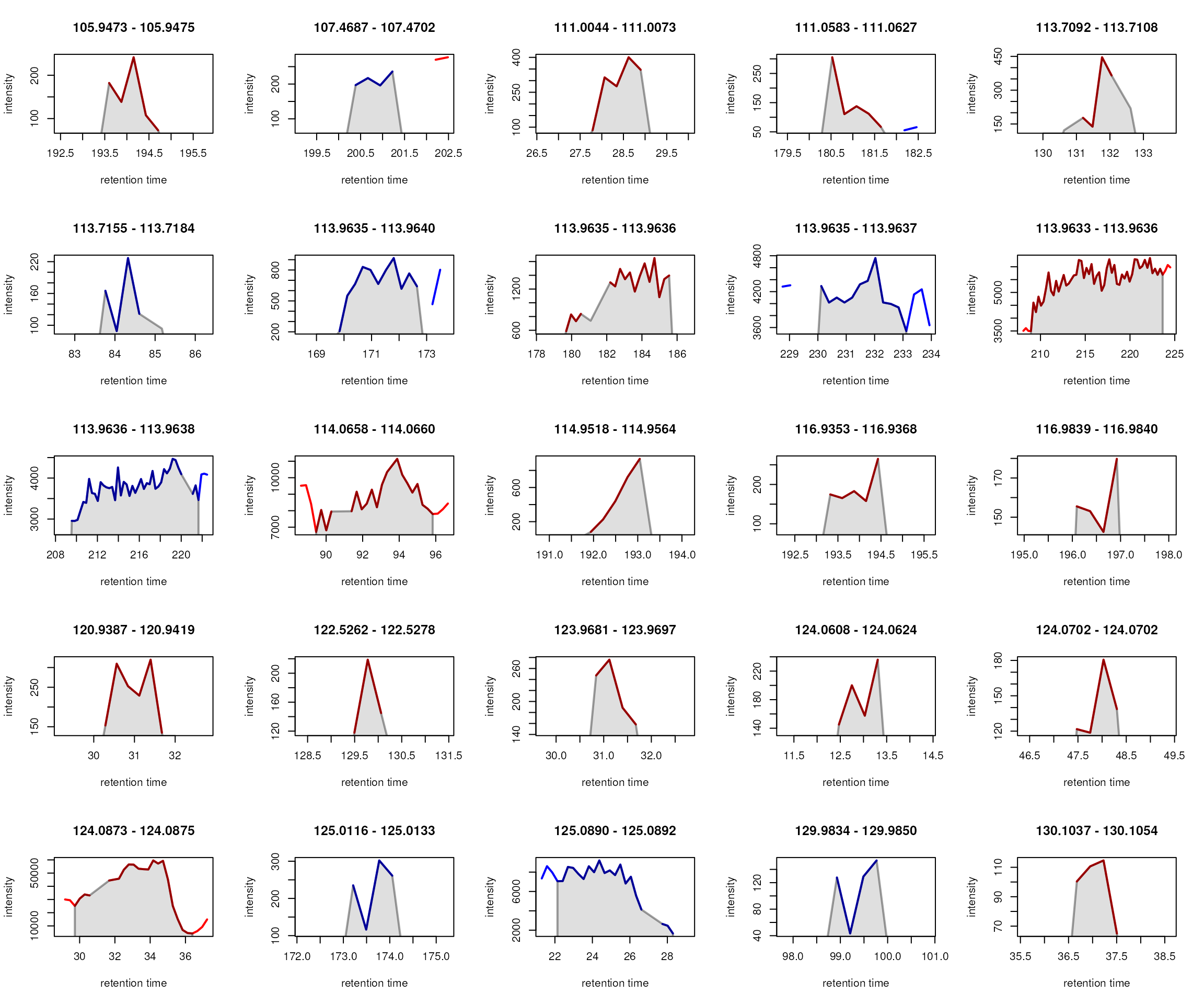
Features with missing values even after gap-filling.
For these features indeed signal was measured only in one of the two samples.
An alternative way to confirm if gap-filling was able to correctly rescue signals is to plot, for features with at least one missing value, the average detected against the average filled-in signal. Ideally, this should be done on QC samples or other repeatedly measured samples were no difference in feature abundances between samples is expected.
The code below extracts first only the detected feature values (by
setting filled = FALSE in the featureValues()
call), then the detected and filled-in signal. For the
latter, the detected signal is subsequently replaced with
NA to create a data matrix with only filled-in values.
Finally, after calculating the row averages for both matrices (excluding
missing values), these values are plotted against each other.
#' Get only detected signal
vals_detect <- featureValues(mse, filled = FALSE)

#' Get detected and filled-in signal
vals_filled <- featureValues(mse)

#' Replace detected signal with NA
vals_filled[!is.na(vals_detect)] <- NA

#' Identify features with at least one filled peak
has_filled <- is.na(rowSums(vals_detect))

#' Calculate row averages
avg_detect <- rowMeans(vals_detect, na.rm = TRUE)
avg_filled <- rowMeans(vals_filled, na.rm = TRUE)

#' Restrict to features with at least one filled peak
avg_detect <- avg_detect[has_filled]
avg_filled <- avg_filled[has_filled]

#' plot the values against each other (in log2 scale)
plot(log2(avg_detect), log2(avg_filled),
     xlim = range(log2(c(avg_detect, avg_filled)), na.rm = TRUE),
     ylim = range(log2(c(avg_detect, avg_filled)), na.rm = TRUE),
     pch = 21, bg = "#00000080")
grid()
abline(0, 1)
Detected (x-axis) against filled (y-axis) signal. The black solid line represents the identity line.
As expected, detected signal is generally higher than filled-in signal. For the biggest part (in particular for higher intensities), filled-in and detected feature values are similar suggesting that the gap filling step indeed rescued signal.
We could also calculate statistics on these values. Below we fit a linear regression line to the data and summarize its result.
##
## Call:
## lm(formula = log2(avg_filled) ~ log2(avg_detect))
##
## Residuals:
##     Min      1Q  Median      3Q     Max
## -4.4598 -0.3337  0.2518  0.7176  1.6402
##
## Coefficients:
##                  Estimate Std. Error t value Pr(>|t|)
## (Intercept)      -1.34738    0.48180  -2.797  0.00613 **
## log2(avg_detect)  1.01347    0.04751  21.333  < 2e-16 ***
## ---
## Signif. codes:  0 '***' 0.001 '**' 0.01 '*' 0.05 '.' 0.1 ' ' 1
##
## Residual standard error: 1.114 on 106 degrees of freedom
##   (25 observations deleted due to missingness)
## Multiple R-squared:  0.8111, Adjusted R-squared:  0.8093
## F-statistic: 455.1 on 1 and 106 DF,  p-value: < 2.2e-16
With a value of 1.007, the slope of the line is thus very close to the slope of the identity line and the two sets of values are also highly correlated (R squared of 0.81).
Preprocessing result
The xcms preprocessing results are all stored within an
XcmsExperiment object. This includes the identified
chromatographic peaks, the alignment results as well as the
correspondence results. In addition, to guarantee reproducibility, this
result object keeps track of all performed processing steps and contains
also the individual parameter objects used in the various preprocessing
steps. These can be extracted with the processHistory()
function:
#' Process history
processHistory(mse)
## [[1]]
## Object of class "XProcessHistory"
## type: Peak detection
## date: Fri Dec 12 08:41:06 2025
## info:
## fileIndex: 1,2
## Parameter class: CentWaveParam
## MS level(s) 1
##
## [[2]]
## Object of class "XProcessHistory"
## type: Peak refinement
## date: Fri Dec 12 08:41:08 2025
## info:
## fileIndex: 1,2
## Parameter class: MergeNeighboringPeaksParam
## MS level(s) 1
##
## [[3]]
## Object of class "XProcessHistory"
## type: Peak grouping
## date: Fri Dec 12 08:41:10 2025
## info:
## fileIndex: 1,2
## Parameter class: PeakDensityParam
## MS level(s) 1
##
## [[4]]
## Object of class "XProcessHistory"
## type: Retention time correction
## date: Fri Dec 12 08:41:10 2025
## info:
## fileIndex: 1,2
## Parameter class: PeakGroupsParam
## MS level(s) 1
##
## [[5]]
## Object of class "XProcessHistory"
## type: Peak grouping
## date: Fri Dec 12 08:41:14 2025
## info:
## fileIndex: 1,2
## Parameter class: PeakDensityParam
## MS level(s) 1
##
## [[6]]
## Object of class "XProcessHistory"
## type: Missing peak filling
## date: Fri Dec 12 08:41:16 2025
## info:
## fileIndex: 1,2
## Parameter class: ChromPeakAreaParam
## MS level(s) 1An individual parameter object can be extracted as follows:
#' Peak detection parameters
processHistory(mse)[[1]]@param
## Object of class: CentWaveParam
## Parameters:
## - ppm: [1] 30
## - peakwidth: [1] 2 10
## - snthresh: [1] 10
## - prefilter: [1] 3 100
## - mzCenterFun: [1] "wMean"
## - integrate: [1] 2
## - mzdiff: [1] -0.001
## - fitgauss: [1] FALSE
## - noise: [1] 0
## - verboseColumns: [1] FALSE
## - roiList: list()
## - firstBaselineCheck: [1] TRUE
## - roiScales: numeric(0)
## - extendLengthMSW: [1] FALSE
## - verboseBetaColumns: [1] FALSEThus, the used preprocessing algorithms along with all their settings are reported along with the preprocessing results.
As described above, values for the individual features can be
extracted from the result object with the featureValues()
function and the definition of the features (which could be used for an
initial annotation of the features based on their m/z and/or
retention times) using the featureDefinitions() function.
In addition, the XcmsExperiment result object, through the
internal Spectra object, keeps a link to the full
MS data used for the analysis. For downstream analyses, that don’t need
access to this MS data anymore, the preprocessing results could be
represented equally well using a SummarizedExperiment
object, which is Bioconductor’s standard container for large-scale omics
data. xcms provides with the quantify() function a
convenience function to extract all results from an
XcmsExperiment result object and return it as a
SummarizedExperiment. This function takes the same
parameters than featureValues(), which is also internally
used to extract the feature value matrix.
#' Extract results as a SummarizedExperiment
library(SummarizedExperiment)
res <- quantify(mse, method = "sum")
The sample annotations can now be accessed with the
colData() function and the feature definitions
(i.e. annotation for individual rows/features) with the
rowData() function:
#' Get sample annotations
colData(res)
## DataFrame with 2 rows and 5 columns
## file sample injection_index
## <character> <character> <numeric>
## 20171016_POOL_POS_1_105-134.mzML 20171016_P... POOL_1 1
## 20171016_POOL_POS_3_105-134.mzML 20171016_P... POOL_2 19
## group spectraOrigin
## <character> <character>
## 20171016_POOL_POS_1_105-134.mzML POOL /__w/xcmsT...
## 20171016_POOL_POS_3_105-134.mzML POOL /__w/xcmsT...
#' Get feature annotations
rowData(res)
## DataFrame with 357 rows and 9 columns
## mzmed mzmin mzmax rtmed rtmin rtmax npeaks
## <numeric> <numeric> <numeric> <numeric> <numeric> <numeric> <numeric>
## FT001 105.042 105.042 105.042 167.6896 167.5019 167.8773 2
## FT002 105.042 105.042 105.042 157.7234 157.7234 157.7234 1
## FT003 105.070 105.069 105.070 31.8081 31.6741 31.9421 2
## FT004 105.110 105.110 105.111 63.7504 63.4566 64.0441 2
## FT005 105.473 105.473 105.474 201.5763 201.3706 201.7820 2
## ... ... ... ... ... ... ... ...
## FT353 133.929 133.929 133.929 193.3516 193.322 193.3808 2
## FT354 133.956 133.956 133.956 199.0666 198.990 199.1432 2
## FT355 133.960 133.960 133.961 30.8309 30.821 30.8409 2
## FT356 133.973 133.973 133.973 206.8718 206.405 207.3387 2
## FT357 133.973 133.973 133.973 200.2561 200.256 200.2561 1
## POOL ms_level
## <numeric> <integer>
## FT001 2 1
## FT002 1 1
## FT003 2 1
## FT004 2 1
## FT005 2 1
## ... ... ...
## FT353 2 1
## FT354 2 1
## FT355 2 1
## FT356 2 1
## FT357 1 1The feature values are stored as an assay within the object.
To access that we simply use the assay() function.
##       20171016_POOL_POS_1_105-134.mzML 20171016_POOL_POS_3_105-134.mzML
## FT001                        3202.7445                        2285.2830
## FT002                        3605.3915                        3191.7385
## FT003                         744.8752                        1057.4312
## FT004                       18126.4603                       19369.4039
## FT005                       23243.6129                       31960.3709
## FT006                         671.5842                         617.7545
SummarizedExperiment objects allow also to have multiple
assay-matrices. We could for example, in addition to the full
feature value matrix, also add a second assay with only the signals from
detected chromatographic peaks (i.e. without the gap-filled data).
#' Assign a new assay to the SummarizedExperiment result object
assay(res, "raw_detected") <- featureValues(mse, method = "sum",
                                            filled = FALSE)
The SummarizedExperiment can be subset by rows and/or
columns. Such subset operations will correctly subset row- and column
data as well as all present assay matrices keeping the structure of the
data sub set intact.
#' Subset to the first 10 features
res[1:10, ]
## class: SummarizedExperiment
## dim: 10 2
## metadata(6): '' '' ... '' ''
## assays(2): raw raw_detected
## rownames(10): FT001 FT002 ... FT009 FT010
## rowData names(9): mzmed mzmin ... POOL ms_level
## colnames(2): 20171016_POOL_POS_1_105-134.mzML
## 20171016_POOL_POS_3_105-134.mzML
## colData names(5): file sample injection_index group spectraOriginWhat next?
After preprocessing, the data could be normalized or scaled to remove any technical variances from the data. While a simple e.g. median scaling could be done with a few lines of R code also more advanced (but not always needed) normalization algorithms are available in e.g. Bioconductor’s preprocessCore package.
Differential abundance analysis could be performed using the limma package or with any of the other packages or methods available in R.
As mentioned above, many chromatographic peaks (and subsequently also features) in untargeted metabolomics data sets will represent isotopes or also different ions/adducts of the same compound. The CAMERA package aimed to identify and group such features in a data set. A similar feature grouping (compounding) can also be done for preprocessing results from newer versions of xcms using the MsFeatures package. This package enables grouping of features through a variety of different methods. See also the feature grouping vignette in xcms for more details.
Finally, the MetaboAnnotation package provides functions to assist in the annotation of features from LC-MS as well as LC-MS/MS experiments. These allow to either perform an initial annotation based on m/z values or through a combination of m/z and retention time values. In addition, also annotations based on fragment spectra (if available) are supported (with or without considering in addition the features’ retention times. More information is provided in the MetaboAnnotation vignette or MetaboAnnotation tutorial.
For more information on general MS data analysis in R or spectra similarity calculations can be found in the RforMassSpectrometry book or in the various workshops/tutorials at SpectraTutorials.
Final words
-
xcmsis not a single, monolithic software, but part of a package ecosystem. - Use the infrastructure provided by the RforMassSpectrometry package ecosystem to inspect, explore and summarize the data.
- Unleash the power of R!
- Create own visualization/summarization functions if needed.
- Combine functionalities from different packages.
- Create customized (and reproducible) analysis workflows.
- Don’t use default settings for xcms preprocessing algorithms.
Appendix
Additional analyses performed on chromatographic or spectra data of preprocessing results
While we used the basic functionality from xcms to perform the preprocessing of an LC-MS experiment, more functionality and visualization options would be available in the infrastructure provided through the xcms, Spectra, MsCoreUtils, MetaboCoreUtils and other related Bioconductor packages. It would for example be easily possible to extract specific information for selected chromatographic peaks or LC-MS features from an xcms result object and perform some additional visualizations or analyses on them. AS an example we below first identify chromatographic peaks that would match the m/z of serine.
#' Extract chromatographic peaks matching the m/z of the [M+H]+ of serine
serine_pks <- chromPeaks(mse, mz = serine_mz, ppm = 20)
serine_pks
## mz mzmin mzmax rt rtmin rtmax into intb
## CP167 106.0506 106.0505 106.0506 181.0848 178.5814 187.4950 74181.78 73905.21
## CP512 106.0496 106.0494 106.0508 181.3459 178.5474 187.4925 70373.61 70109.36
## maxo sn sample
## CP167 37664.94 685 1
## CP512 38517.76 830 2The chromPeakChromatograms() function can then be used
to extract the EIC of a specific chromatographic peak in a sample.
#' Extract EIC for the signal in the second sample
serine_eic_2 <- chromPeakChromatograms(mse, peaks = rownames(serine_pks)[2])
We can also extract the full MS1 scan (spectrum) at the apex position
of that chromatographic peak using the chromPeakSpectra()
function with parameters msLevel = 1 and
method = "closest_rt".
# Extract the full MS1 scan for the chrom peak at apex position
serine_ms1_2 <- chromPeakSpectra(mse, msLevel = 1, method = "closest_rt",
                                 peaks = rownames(serine_pks)[2])
For LC-MS/MS data, this function would also allow to extract all MS2
spectra from the data set with their precursor m/z (and retention time)
within the chromatographic peak’s m/z and retention time width
by using parameters msLevel = 2 and
method = "all".
Below we plot the EIC and the MS1 scan for the selected chromatographic peak.
par(mfrow = c(1, 2))

#' Plot the EIC
plot(serine_eic_2)
#' Indicate the retention time of the full scan MS1 spectrum
abline(v = rtime(serine_ms1_2), lty = 2)
#' Plot the full scan MS1 spectrum
plotSpectra(serine_ms1_2)
#' Indicate the theoretical m/z of the
points(serine_mz, y = -300, pch = 2, col = "red")![EIC for the [M+H]+ ion of serine in one sample and full scan MS1 spectrum at the EIC's apex position.](xcms-preprocessing_files/figure-html/unnamed-chunk-67-1.png)
EIC for the [M+H]+ ion of serine in one sample and full scan MS1 spectrum at the EIC’s apex position.
Similar information can also be extracted for LC-MS features using
the featureChromatograms() and
featureSpectra() functions but these functions will return
chromatograms and spectra for all samples in the
experiment (not just for a single sample). Also, importantly, while the
chromPeakChromatogram() extracts the EIC specific for the
selected sample, i.e. using the exact m/z and retention time
ranges of the chromatographic peak in that sample,
featureChrommatograms() will instead integrate the signal
from the m/z and retention time area of the
feature, i.e. will use a single area and integrate the
signal from that same area in each sample. This m/z - retention
time area might however be larger than the respective ranges for a
single chromatographic peak in one sample. This m/z - retention
time area for features can also be extracted (and evaluated) using the
featureArea() function:
#' Extract the m/z - retention time area for features
featureArea(mse) |>
    head()
## mzmin mzmax rtmin rtmax
## FT001 105.0389 105.0448 162.48680 173.03646
## FT002 105.0403 105.0434 154.65033 161.36642
## FT003 105.0680 105.0727 30.56318 34.46556
## FT004 105.1098 105.1114 61.19807 72.20464
## FT005 105.4717 105.4747 198.86525 211.48482
## FT006 105.7141 105.7183 179.69288 182.74128Additional analyses could now be performed on the full scan MS1
spectrum containing a mass peak for the [M+H]+ ion of serine. One
possibility would be to identify potential isotope peaks of the
monoisotopic mass peak of serine. The isotopologues
function from the MetaboCoreUtils
allows for example to identify and group potential isotope peaks in MS1
spectrum data without any assumptions on the chemical formula of the
compound of interest.
#' Extract the mass peak data from the MS1 spectrum containing
#' the signal from an ion of serine
pd <- peaksData(serine_ms1_2)[[1]]
head(pd)
## mz intensity
## [1,] 105.0338 97.01923
## [2,] 105.7157 574.78322
## [3,] 105.7288 137.45455
## [4,] 105.8477 208.91608
## [5,] 105.9348 239.67133
## [6,] 105.9537 196.95804
#' Identify mass peaks that could represent isotopes of the mass peak
#' of the [M+H]+ ion of serine
iso_idx <- isotopologues(pd, seedMz = serine_mz)
iso_idx
## [[1]]
## [1] 8 14The function thus identified two peaks that, based on their m/z values and differences in intensity, could represent isotopologues. We below highlight these mass peaks in the full MS1 spectrum.
#' Set the color for each mass peak to a transparent black color
cols <- rep("#00000040", lengths(serine_ms1_2)[1])
#' Use a red color for the identified isotopologues
cols[iso_idx[[1]]] <- "#ff0000ff"
#' Plot the data
plotSpectra(serine_ms1_2, col = cols, lwd = 2)![Full scan spectrum at apex position of the signal for the [M+H]+ ion for serine. Isotopologues are indicated in red.](xcms-preprocessing_files/figure-html/unnamed-chunk-70-1.png)
Full scan spectrum at apex position of the signal for the [M+H]+ ion for serine. Isotopologues are indicated in red.
While in the example above we were specifically looking for potential
isotopes of a single, selected, mass peak (by setting
seedMz to the m/z value of that peak), we could
also use isotopologues() without specifying
seedMz to identify all potential isotope groups in a
spectrum.
#' Identify all potential isotope peaks in the MS1 spectrum
iso_idx <- isotopologues(pd)
iso_idx
## [[1]]
## [1] 3 17
##
## [[2]]
## [1] 8 14
##
## [[3]]
## [1] 34 40 43
##
## [[4]]
## [1] 42 50
##
## [[5]]
## [1] 66 74
##
## [[6]]
## [1] 78 85 88
##
## [[7]]
## [1] 100 104
##
## [[8]]
## [1] 109 121We can also highlight these in the spectrum plot.
#' Define a color for all mass peaks and set it to transparent black
cols <- rep("#00000040", lengths(serine_ms1_2)[1])
#' Use a different color for each isotope group
iso_cols <- rainbow(length(iso_idx))
for (i in seq_along(iso_idx))
    cols[iso_idx[[i]]] <- iso_cols[i]
plotSpectra(serine_ms1_2, col = cols, lwd = 2)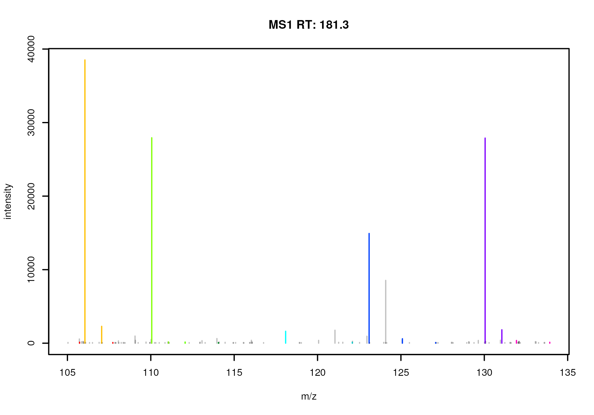
MS1 spectrum with potential isotope groups highlighted in different colors.
Note that such isotopologue identification is not limited to data
from a MS1 spectrum. We could also identify features representing signal
from potential isotopes. For this we below create a matrix
with the features’ m/z values and the maximum intensity of the
feature in one of the samples and apply the isotopologues()
function on it.
#' Define a matrix with the m/z and intensity values for each feature.
#' As intensity we use the highest measured intensity in the first
#' sample
pd <- cbind(
    mz = featureDefinitions(mse)$mzmed,
    intensity = featureValues(mse, value = "maxo")[, 1]
)
#' Ensure the matrix to be sorted by m/z value
pd <- pd[order(pd[, "mz"]), ]

#' Identify potential isotope groups
iso_idx <- isotopologues(pd)

head(iso_idx)
## [[1]]
## FT015
## 9 15
##
## [[2]]
## FT012
## 10 12
##
## [[3]]
## FT023 FT046
## 13 23 46
##
## [[4]]
## FT035
## 24 35
##
## [[5]]
## FT040 FT060 FT069
## 29 40 60 69
##
## [[6]]
## FT061 FT087
## 31 61 87We thus identified potential isotopologues, but, because we ignored the retention times of the features in this simple approach, the list will contain also many false positives. The features of the isotope group below for example all have different retention times and can thus not represent signal from isotopes of the same compound.
#' Show a false positive finding
featureDefinitions(mse)[iso_idx[[3]], ]
## mzmed mzmin mzmax rtmed rtmin rtmax npeaks POOL
## FT013 107.0654 107.0653 107.0656 173.2621 173.2108 173.3134 2 2
## FT023 109.0634 109.0632 109.0636 161.6905 161.6466 161.7343 2 2
## FT046 111.0601 111.0601 111.0601 181.0848 181.0848 181.0848 1 1
## peakidx ms_level
## FT013 132, 429 1
## FT023 76, 374 1
## FT046 140 1Others however could be real isotopes:
featureDefinitions(mse)[iso_idx[[2]], ]## mzmed mzmin mzmax rtmed rtmin rtmax npeaks POOL
## FT010 106.0501 106.0496 106.0506 181.2154 181.0848 181.3459 2 2
## FT012 107.0535 107.0532 107.0538 181.2154 181.0848 181.3459 2 2
## peakidx ms_level
## FT010 153, 461 1
## FT012 143, 444 1Additional visualizations
Visualization is key to understand the signal measured by an MS instrument and also to evaluate the performance (and quality) of the preprocessing. However, LC-MS data is particularly difficult to visualize because of its 3-dimensional nature. Focusing on specific m/z - retention time ranges (EICs) can help, but provides only information on small subsets of the whole data. In this section we present an alternative approach to visualize the whole chromatographic peak space from an LC-MS experiment.
We below subset the data to the first sample and visualize the
identified chromatographic peaks in the m/z - retention time
plane using the plotChromPeaks() function that we used
already before.
#' Plot identified chromatographic peaks in the first sample
mse_1 <- mse[1]
plotChromPeaks(mse_1)
Position of identified chromatographic peaks in the first sample.
While this plot provides information on the region in which peaks
were identified and on the retention time widths of the peaks, it does
not allow to investigate peak shapes or intensities. Such information
would be provided (for a single ion) by an extracted ion chromatogram.
We thus below extract ion chromatograms for every identified
chromatographic peak in the first sample. With parameter
expandRt = 4 we increase for each chromatographic peak the
region from which the data will be extracted by 4 seconds on either
side.
#' Extract EICs for each identified chromatographic peak
chrs_all <- chromPeakChromatograms(mse_1, expandRt = 4)
While we could now simply proceed and plot each of the 356 EICs
separately, we instead use below the
plotChromatogramsOverlay() function that allows to plot
multiple EICs into the same plot hence providing an overview of the full
set of identified chromatographic peaks. By setting parameter
stacked to a value different then 0 it is
possible to stack the chromatograms along the y-axis hence
providing a simple 3-dimensional impression of the data. For easier
visualization we in addition increase the transparency of the colors for
the individual lines (parameter col), and the identified
chromatographic peaks (parameter peakCol and
peakBg for the foreground and background color,
respectively).
#' Create a stacked EIC plot
plotChromatogramsOverlay(chrs_all, stacked = 1, bty = "n",
                         col = "#00000020", peakCol = "#00000020",
                         peakBg = "#00000020")
All identified chromatographic peaks in one sample shown as a pseudo 3-dimensional plot.
This plot thus provides a general overview of the detected signal (chromatographic peaks) of a data file. We can immediately spot some very high intensity peaks, regions with higher number of ions and also signal from potential contaminants.
Instead of the full data range we can also zoom into a region and extract EICs from that for a closer inspection of the data. Below we define an area from a m/z value from 113 to 119 and a retention time from 125 to 145 seconds.
#' Plot location of all peaks and highlight region of interest
plotChromPeaks(mse_1)
rect(125, 113, 145, 119, lty = 3, border = "#ff000080", lwd = 2)
Selected region from which EICs should be extracted and plotted.
With the m/z ranges from the chromatographic peaks in that region defined, we can next extract ion chromatograms for the data slices defined by these m/z ranges and the selected (fixed) retention time range.
#' Extract chrom peaks from that region
pks <- chromPeaks(mse_1, mz = c(113, 119), rt = c(125, 145))

#' Extract EICs for the m/z slices of the chromatographic peaks
#' and the full retention time window of the area
chrs_sub <- chromatogram(mse_1, mz = pks[, c("mzmin", "mzmax")],
                         rt = cbind(rep(125, nrow(pks)),
                                    rep(145, nrow(pks))))
We can now plot the EICs from that region again using the
plotChromatogramsOverlay() function. Next to plotting the
data, this function also silently returns the y-positions of the
individual EICs in the plot. We assign that below to a variable
y and use this information to draw the m/z for the
EICs along the y-axis.
#' Plot the EICs of the selected area
y <- plotChromatogramsOverlay(chrs_sub, stacked = 1, bty = "n",
                              col = "#00000020", peakCol = "#00000020",
                              peakBg = "#00000020")

#' Draw horizonal lines
abline(h = y[[1]], col = "#00000020", lty = 3)
#' Add m/z values of the EICs to the plot
mzs <- format(rowMeans(mz(chrs_sub)), digits = 5)
text(x = rep(126, length(mzs)), y = y[[1]],
     labels = paste0("m/z = ", mzs), pos = 1)
EICs from a selected m/z - retention time region.
Some of the EICs seem to represent signals from isotopes (e.g. the
EIC at 114.07 and 115.07). In fact, we can again use the
isotopologues() function from the MetaboCoreUtils
to check whether pairs of m/z and intensity values would match
signal expected for isotopes.
#' Order the extracted chromatographic peaks by m/z
pks <- pks[order(pks[, "mz"]), ]

#' Test which signals could come from isotopes
isotopologues(pks[, c("mz", "into")])
## [[1]]
## CP053
## 2 3
##
## [[2]]
## CP054
## 4 5Pairs of chromatographic peaks have been identified as being potential isotopologues.
Bonus material - peak detection fun
In this section we apply the lessons learned from previous sections, in particular how to adapt peak detection setting on a rather noisy chromatographic data. Below we load the example data from a text file.
cdata <- read.table(
    system.file("txt", "chromatogram.txt", package = "xcmsTutorials"),
    sep = "\t", header = TRUE)
head(cdata)
## rt intensity
## 1 100 0
## 2 110 0
## 3 120 1
## 4 130 2
## 5 140 4
## 6 150 6Our data has two columns, one with retention times and one
with intensities. We can now create a Chromatogram
object from that and plot the data.
library(MSnbase)
chr <- Chromatogram(rtime = cdata$rt, intensity = cdata$intensity)
par(mar = c(2, 2, 0, 0))
plot(chr)
There are two peaks present in the data, with the signal from the
latter being particularly noisy. The goal is now to perform the peak
detection and to identify the two peaks. A first try with the default
settings for centWave clearly shows that we have to tune the
parameters (note that the setting of sn = 0 is required for
the present data set as there are not enough background data
points for the algorithm to estimate the noise level properly).
Which parameter would you now adapt to the data? What would be your
choices? Go ahead and try different settings or setting combination to
see if you can succeed in detecting the two peaks. Eventually you might
even try a different peak detection algorithm
(e.g. MatchedFilterParam).
xchr <- findChromPeaks(chr, param = CentWaveParam(sn = 0))
par(mar = c(2, 2, 0, 0))
plot(xchr)
With the default parameters centWave clearly failed to identify the two large peaks, defining only smaller fragments of them as potential peaks. Especially the second peak with its peculiar tri-forked shape seems to cause troubles. This would be even for a hydrophilic liquid interaction chromatography (HILIC), known to potentially result in noisy odd-shaped peaks, a rather unusual peak shape. In fact, the signal we were analyzing here is not of chromatographic origin:

Our example data represents a panorama picture featuring mountains from the Dolomites, the Paternkofel (left peak, colored red) and the famous Drei Zinnen (right tri-forked peak colored green).
Session information
## R version 4.5.2 (2025-10-31)
## Platform: x86_64-pc-linux-gnu
## Running under: Ubuntu 24.04.3 LTS
##
## Matrix products: default
## BLAS:   /usr/lib/x86_64-linux-gnu/openblas-pthread/libblas.so.3
## LAPACK: /usr/lib/x86_64-linux-gnu/openblas-pthread/libopenblasp-r0.3.26.so;  LAPACK version 3.12.0
##
## locale:
##  [1] LC_CTYPE=en_US.UTF-8       LC_NUMERIC=C
##  [3] LC_TIME=en_US.UTF-8        LC_COLLATE=en_US.UTF-8
##  [5] LC_MONETARY=en_US.UTF-8    LC_MESSAGES=en_US.UTF-8
##  [7] LC_PAPER=en_US.UTF-8       LC_NAME=C
##  [9] LC_ADDRESS=C               LC_TELEPHONE=C
## [11] LC_MEASUREMENT=en_US.UTF-8 LC_IDENTIFICATION=C
##
## time zone: Etc/UTC
## tzcode source: system (glibc)
##
## attached base packages:
## [1] stats4    stats     graphics  grDevices utils     datasets  methods
## [8] base
##
## other attached packages:
##  [1] RColorBrewer_1.1-3          png_0.1-8
##  [3] MSnbase_2.36.0              mzR_2.44.0
##  [5] Rcpp_1.1.0                  SummarizedExperiment_1.40.0
##  [7] Biobase_2.70.0              GenomicRanges_1.62.1
##  [9] Seqinfo_1.0.0               IRanges_2.44.0
## [11] MatrixGenerics_1.22.0       matrixStats_1.5.0
## [13] MetaboCoreUtils_1.18.1      pheatmap_1.0.13
## [15] Spectra_1.20.0              S4Vectors_0.48.0
## [17] BiocGenerics_0.56.0         generics_0.1.4
## [19] MsExperiment_1.12.0         ProtGenerics_1.42.0
## [21] xcms_4.8.0                  BiocParallel_1.44.0
## [23] rmarkdown_2.30              knitr_1.50
## [25] BiocStyle_2.38.0
##
## loaded via a namespace (and not attached):
##  [1] DBI_1.2.3                   rlang_1.1.6
##  [3] magrittr_2.0.4              clue_0.3-66
##  [5] MassSpecWavelet_1.76.0      compiler_4.5.2
##  [7] systemfonts_1.3.1           vctrs_0.6.5
##  [9] reshape2_1.4.5              stringr_1.6.0
## [11] crayon_1.5.3                pkgconfig_2.0.3
## [13] fastmap_1.2.0               XVector_0.50.0
## [15] preprocessCore_1.72.0       ragg_1.5.0
## [17] purrr_1.2.0                 xfun_0.54
## [19] MultiAssayExperiment_1.36.1 cachem_1.1.0
## [21] jsonlite_2.0.0              progress_1.2.3
## [23] DelayedArray_0.36.0         prettyunits_1.2.0
## [25] parallel_4.5.2              cluster_2.1.8.1
## [27] R6_2.6.1                    bslib_0.9.0
## [29] stringi_1.8.7               limma_3.66.0
## [31] jquerylib_0.1.4             iterators_1.0.14
## [33] bookdown_0.46               BiocBaseUtils_1.12.0
## [35] Matrix_1.7-4                igraph_2.2.1
## [37] tidyselect_1.2.1            abind_1.4-8
## [39] yaml_2.3.12                 doParallel_1.0.17
## [41] codetools_0.2-20            affy_1.88.0
## [43] lattice_0.22-7              tibble_3.3.0
## [45] plyr_1.8.9                  S7_0.2.1
## [47] evaluate_1.0.5              desc_1.4.3
## [49] pillar_1.11.1               affyio_1.80.0
## [51] BiocManager_1.30.27         foreach_1.5.2
## [53] MALDIquant_1.22.3           ncdf4_1.24
## [55] hms_1.1.4                   ggplot2_4.0.1
## [57] scales_1.4.0                glue_1.8.0
## [59] MsFeatures_1.18.0           lazyeval_0.2.2
## [61] tools_4.5.2                 mzID_1.48.0
## [63] data.table_1.17.8           QFeatures_1.20.0
## [65] vsn_3.78.0                  fs_1.6.6
## [67] XML_3.99-0.20               grid_4.5.2
## [69] impute_1.84.0               tidyr_1.3.1
## [71] MsCoreUtils_1.22.1          PSMatch_1.14.0
## [73] cli_3.6.5                   textshaping_1.0.4
## [75] S4Arrays_1.10.1             dplyr_1.1.4
## [77] AnnotationFilter_1.34.0     pcaMethods_2.2.0
## [79] gtable_0.3.6                sass_0.4.10
## [81] digest_0.6.39               SparseArray_1.10.6
## [83] htmlwidgets_1.6.4           farver_2.1.2
## [85] htmltools_0.5.9             pkgdown_2.2.0
## [87] lifecycle_1.0.4             statmod_1.5.1
## [89] MASS_7.3-65
Acknowledgments
Thank you to Philippine Louail for fixing typos and suggesting improvements.