library(MsExperiment)     # container for MS data
library(Spectra)          # main MS infrastructure for R
library(xcms)             # for preprocessing of LC-MS and LC-MS/MS data
library(MsBackendMassIVE) # to load MS data directly from MassIVE
library(MsBackendMgf)     # to export MS data in MGF format

library(RColorBrewer) # to define colors
library(pander)       # to format tables
library(pheatmap)     # visualization of clustering results as heatmap
library(vioplot) # to create *violin plots*xcms-based Preprocessing of LC-MS/MS Data for Feature-Based Molecular Networking with GNPS2
Source:vignettes/MSV000090156-preprocessing.qmd
Introduction
This document describes data inspection and preprocessing of an LC-MS/MS data set using xcms (Louail, Brunius, et al. 2025) and export of the data for subsequent feature-based molecular networking (FBMN) with GNPS2. Functionality from different packages from the RforMassSpectrometry package ecosystem are combined to visualize and process the data.
For details and more in depth description of the various visualizations and analysis options as well as parameter choices see also the Metabonaut tutorials (Louail, Graeve, et al. 2025).
This analysis and the used settings should be considered initial with potential refinement and improvement based on discussions expected during integration of the analysis into the FBMN workflow.
Required software packages
The various software packages required for the analysis are defined and loaded below. All packages are available through Bioconductor or CRAN and can be installed with BiocManager::install(<package name>).
ℹ️ Note
MsBackendMassIVE is currently (as of 2026-06) available only in the developmental branch of Bioconductor and needs to be installed from GitHub using
remotes::install_github("RforMassSpectrometry/MsBackendMassIVE").
Data import
The data analyzed here is part of the MassIVE MSV000090156 data set. Here we will analyze the data from Lab 2. Rather than downloading the raw mzML files manually, we use the MsBackendMassIVE backend, which fetches the MS data files directly from the MassIVE FTP server and caches them locally via BiocFileCache, so subsequent runs do not re-download anything.
Before loading the data we define a data.frame with sample and experiment-specific information for the individual MS runs/data files. These should ideally comprise all relevant phenotypic but also technical information (e.g. injection index) to allow proper adjusting or modeling of the data.
pd <- data.frame(
    original_file_name = c("Interlab-LC-MS_Lab2_A15M_Pos_MS2_Rep1.mzML",
                           "Interlab-LC-MS_Lab2_A15M_Pos_MS2_Rep2.mzML",
                           "Interlab-LC-MS_Lab2_A15M_Pos_MS2_Rep3.mzML",
                           "Interlab-LC-MS_Lab2_A45M_Pos_MS2_Rep1.mzML",
                           "Interlab-LC-MS_Lab2_A45M_Pos_MS2_Rep2.mzML",
                           "Interlab-LC-MS_Lab2_A45M_Pos_MS2_Rep3.mzML",
                           "Interlab-LC-MS_Lab2_A5M_Pos_MS2_Rep1.mzML",
                           "Interlab-LC-MS_Lab2_A5M_Pos_MS2_Rep2.mzML",
                           "Interlab-LC-MS_Lab2_A5M_Pos_MS2_Rep3.mzML",
                           "Interlab-LC-MS_Lab2_M_Pos_MS2_Rep1.mzML",
                           "Interlab-LC-MS_Lab2_M_Pos_MS2_Rep2.mzML",
                           "Interlab-LC-MS_Lab2_M_Pos_MS2_Rep3.mzML",
                           "Interlab-LC-MS_Lab2_PPL_Pos_MS2_Rep1.mzML"),
    sample_name = c("A15M", "A15M", "A15M",
                    "A45M", "A45M", "A45M",
                    "A5M", "A5M", "A5M",
                    "M", "M", "M",
                    "PPL"),
    sample_desc = c("A15M_R1", "A15M_R2", "A15M_R3",
                    "A45M_R1", "A45M_R2", "A45M_R3",
                    "A5M_R1", "A5M_R2", "A5M_R3",
                    "M_R1", "M_R2", "M_R3",
                    "PPL_R1"),
    replicate = c(1, 2, 3, 1, 2, 3, 1, 2, 3, 1, 2, 3, 1)
)
We next load the Lab 2 mzML files of the data set directly from MassIVE. The filePattern argument is used to restrict the download to the 13 Lab 2 mzML files. The first call will download (and cache) the files; subsequent calls will simply reload them from the local cache.
#' Load the Lab 2 mzML files from MassIVE (downloaded & cached on first run)
sps <- Spectra("MSV000090156",
               filePattern = "Lab_2/Interlab-LC-MS_Lab2.*mzML$",
               source = MsBackendMassIVE())

#' Helper sample data column and spectra variable used to link spectra to
#' samples in `pd`
pd$file_name <- paste0("MSV000090156_", pd$original_file_name)
sps$file_name <- basename(dataOrigin(sps))

#' Wrap into an MsExperiment and link sample data to spectra by file name
mse <- MsExperiment(spectra = sps,
                    sampleData = DataFrame(pd))
mse <- linkSampleData(mse,
                      with = "sampleData.file_name = spectra.file_name")
mse
Object of class MsExperiment
Spectra: MS1 (16302) MS2 (49500)
Experiment data: 13 sample(s)
Sample data links:
- spectra: 13 sample(s) to 65802 element(s).The samples and data files from the present data set are displayed in the table below. Note that in the R code block below we use the R pipe operator |> to avoid nested function calls and improve the readability of the code.
sampleData(mse)[, c("sample_name", "sample_desc", "replicate")] |>
    as.data.frame() |>
pandoc.table(style = "rmarkdown", split.table = Inf)| sample_name | sample_desc | replicate |
|---|---|---|
| A15M | A15M_R1 | 1 |
| A15M | A15M_R2 | 2 |
| A15M | A15M_R3 | 3 |
| A45M | A45M_R1 | 1 |
| A45M | A45M_R2 | 2 |
| A45M | A45M_R3 | 3 |
| A5M | A5M_R1 | 1 |
| A5M | A5M_R2 | 2 |
| A5M | A5M_R3 | 3 |
| M | M_R1 | 1 |
| M | M_R2 | 2 |
| M | M_R3 | 3 |
| PPL | PPL_R1 | 1 |
We in addition also define different colors for the individual samples.
#' Define a color for each unique original sample
col <- sampleData(mse)$sample_name |>
                     unique() |>
                     length() |>
                     brewer.pal("Set2")
names(col) <- unique(sampleData(mse)$sample_name)

#' Define a color for each data file/sample
col_sample <- col[sampleData(mse)$sample_name]
Data visualization and general quality assessment
For data inspection and a general data overview we first create base peak chromatograms (BPC) and total ion chromatograms (TIC) of the data set using the chromatograms() functions specifying either "max" (for BPC) or "sum" (for TIC) as the function to aggregate the per-spectrum intensities.
#' BPC
bpc <- chromatogram(mse, aggregationFun = "max")

plot(bpc, col = paste0(col_sample, 80), main = "BPC", lwd = 2)
grid()
legend("topright", col = col, legend = names(col), lty = 1, lwd = 2)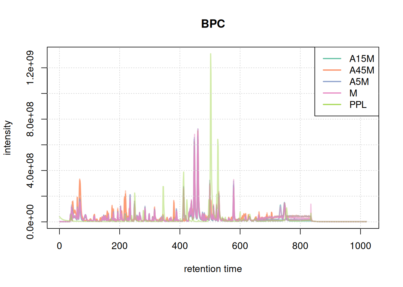
#' TIC
tic <- chromatogram(mse, aggregationFun = "sum")

plot(tic, col = paste0(col_sample, 80), main = "TIC", lwd = 2)
grid()
legend("topright", col = col, legend = names(col), lty = 1, lwd = 2)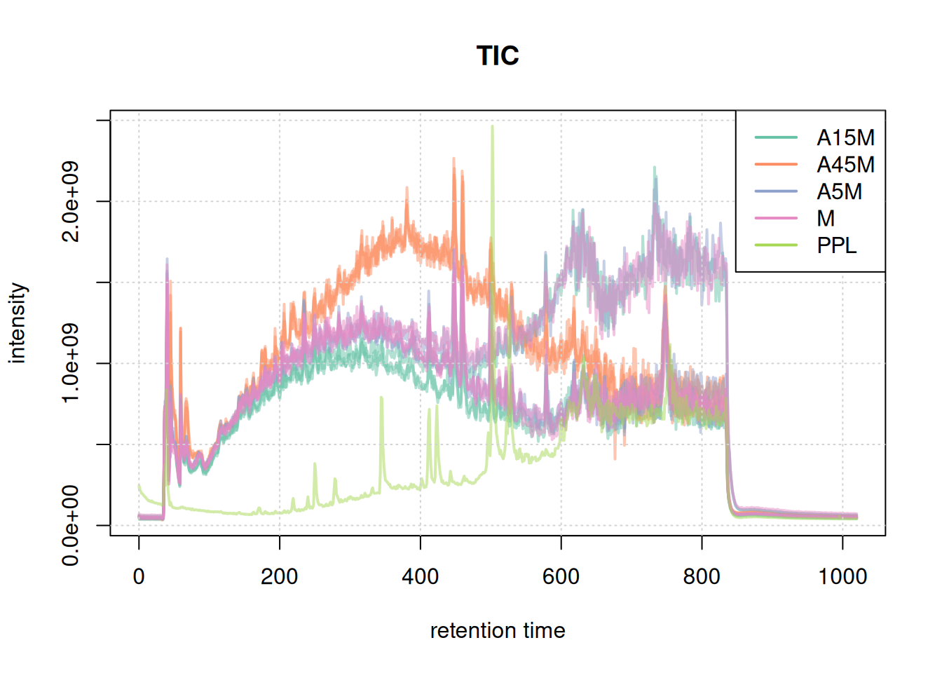
Based on the BPC and TIC there seems to be little retention time shifts between the samples. Also, no signal seems to be present before 20 seconds and after 850 seconds. Thus, we below filter the data set to spectra acquired within this retention time range.
#' filter the data set to a retention time range from 20 to 850 seconds
mse <- filterSpectra(mse, filterRt, c(20, 850))
BPC and TIC aggregate data along the m/z dimension per spectrum (retention time) to compare the signal measured along the retention time. To compare the mass or ion content of the individual samples/measurement runs we in addition aggregate data along the retention time, for distinct m/z values.
To this end we first bin each spectrum to get discrete and similar m/z values within the data set.
#' bin mass peaks into into discrete m/z bins of 0.02 Da.
s_bin <- spectra(mse) |>
    filterMsLevel(1L) |>
    bin(binSize = 0.02)

#' combine all spectra within the same sample into a single spectrum
#' reporting the maximum intensity of all mass peaks with the same m/z bin
bps <- combineSpectra(s_bin, f = s_bin$dataOrigin, intensityFun = max)
#' the same but reporting the sum of intensities per m/z bin
tis <- combineSpectra(s_bin, f = s_bin$dataOrigin, intensityFun = sum)
We have thus a single aggregated mass spectrum per sample. These base peak spectra are plotted below.
par(mar = c(4.5, 4, 0, 0.5))
plotSpectra(bps, main = "")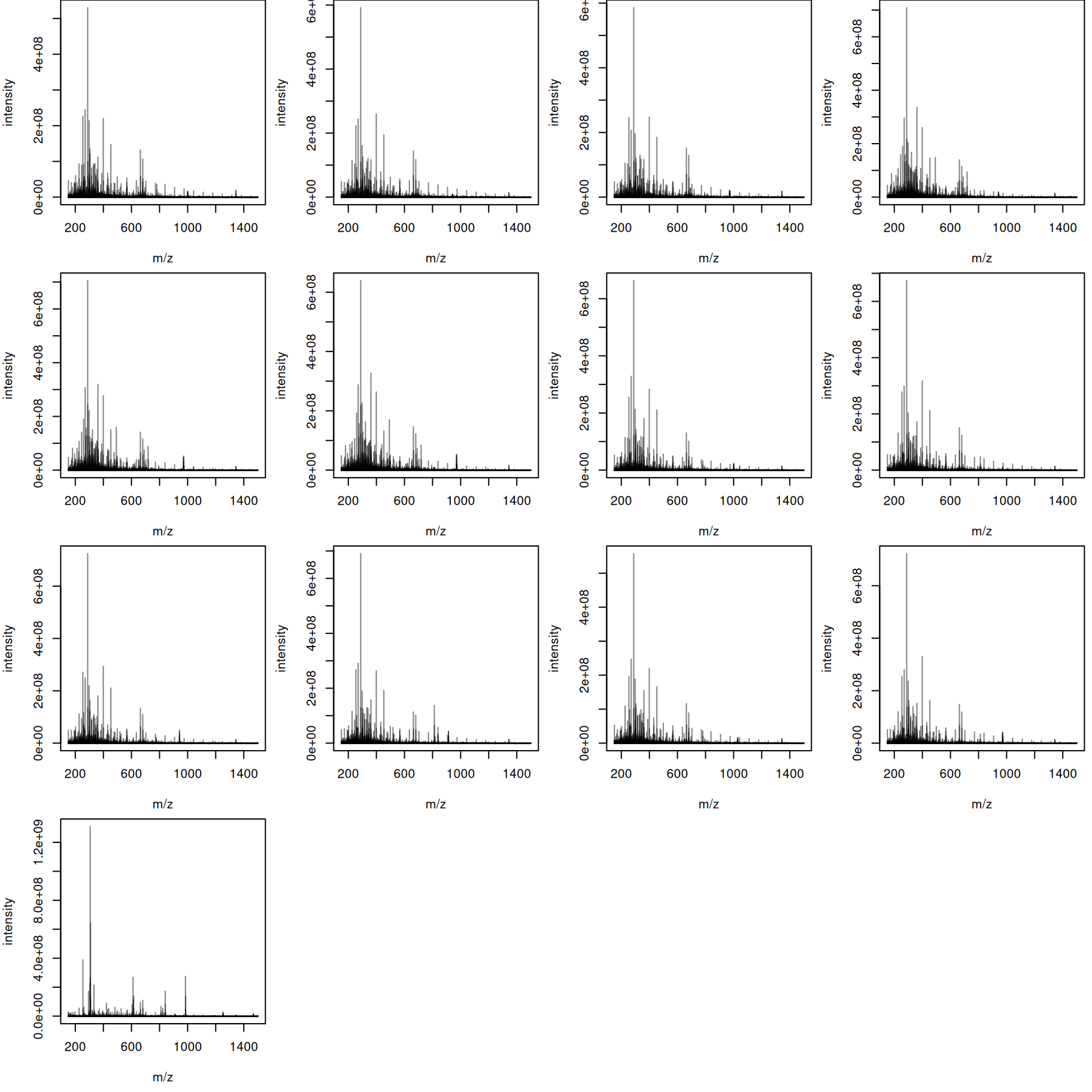
The mass content of the samples seems to be similar, with the exception of the last file. We can also plot all spectra into the same plot, using a different color per sample.
plotSpectraOverlay(bps, col = paste0(col_sample, 40), lwd = 2)
grid()
legend("topright", col = col, legend = names(col), lty = 1)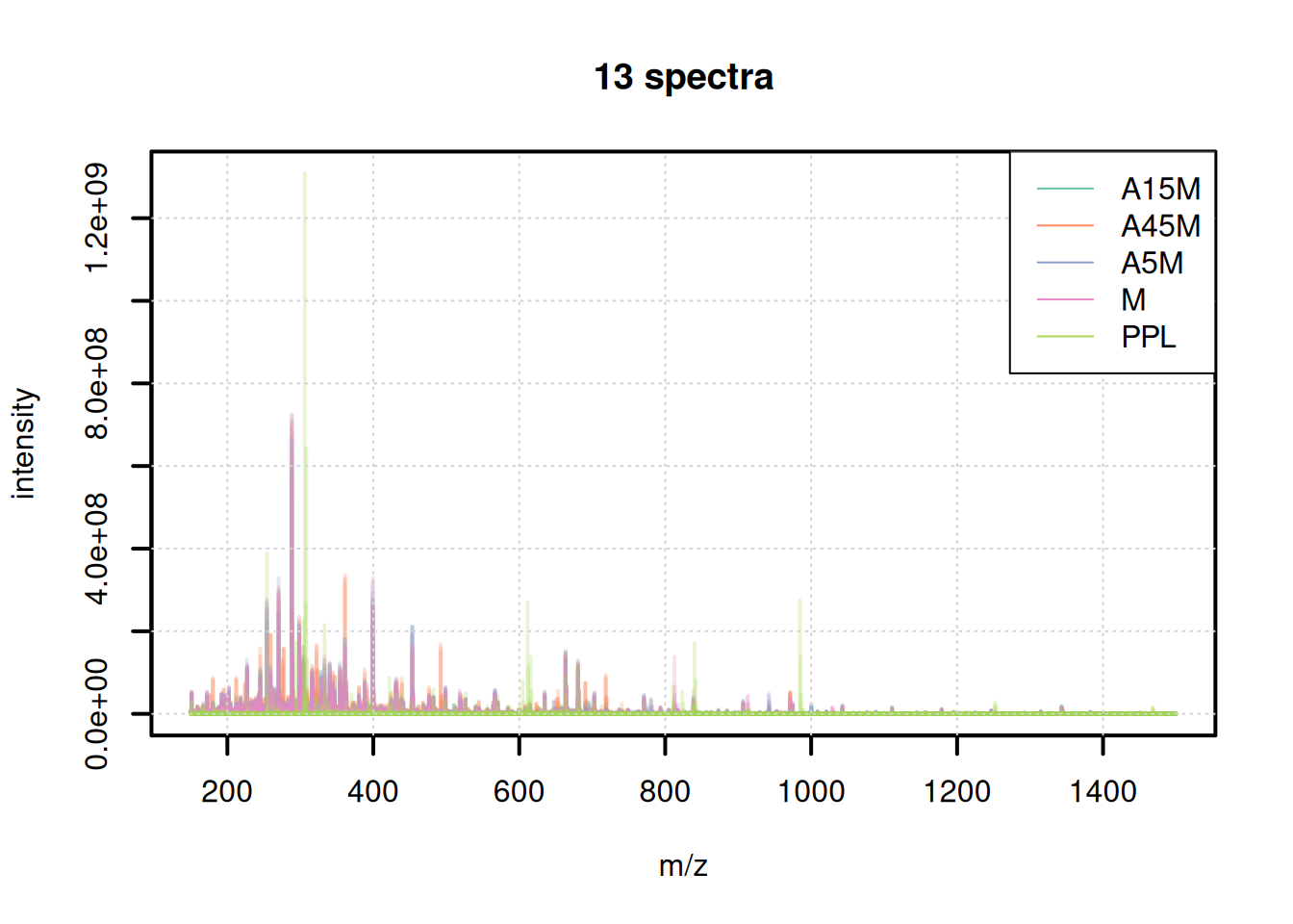
The mass content seems to be comparable between samples, except for the PPM sample that shows distinct peaks.
For a more quantitative assessment and comparison we can also use these calculate a spectra similarity between these aggregated spectra to calculate spectra similarity between the individual samples and cluster them.
sim <- compareSpectra(bps)
rownames(sim) <- colnames(sim) <- sampleData(mse)$sample_desc
pheatmap(sim)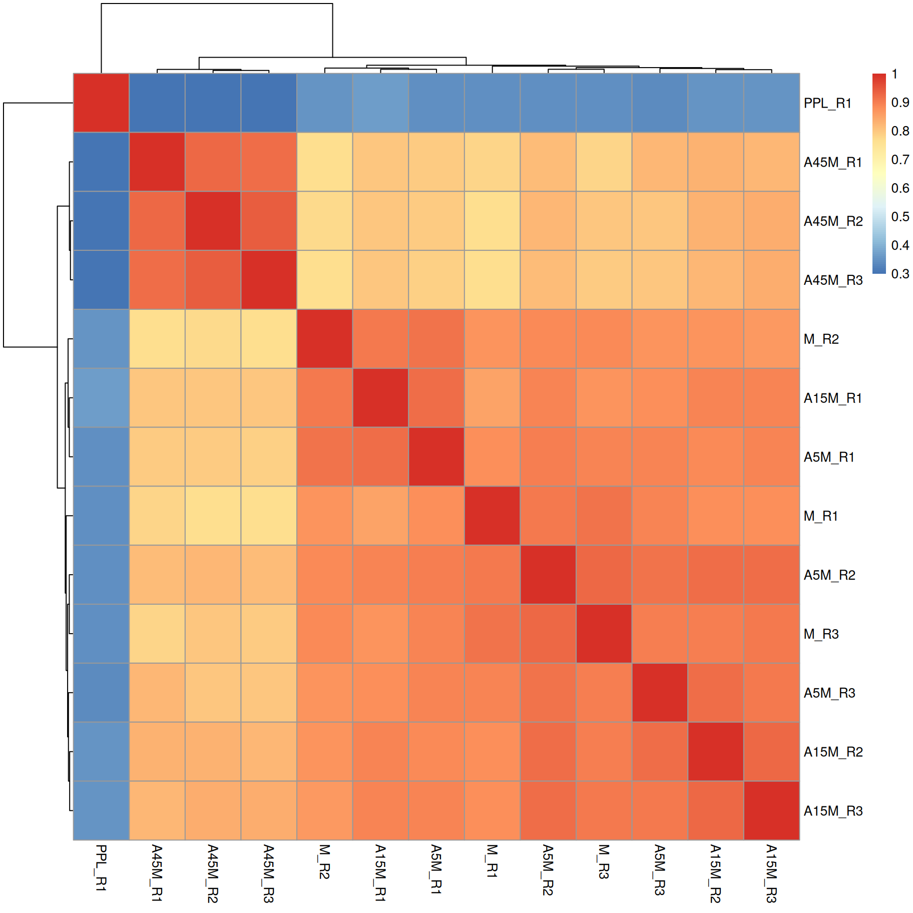
A15M, A5M and M samples cluster together, separately from the A45M samples while the PPL_R1 sample has a distinct mass peak profile.
Data preprocessing
Data preprocessing is the first step in the analysis of LC-MS data processing and analyzing the raw MS data to result in a two-dimensional quantification table of LC-MS features in the various samples of the experiment. This process consists of 3 main steps: chromatographic peak detection, retention time alignment and correspondence analysis. An additional gap-filling step can be conducted to reduce the number of missing values integrating raw MS signal from the expected m/z by retention time areas of defined LC-MS features.
Most methods in xcms are parallelized by default. Below we define the parallel processing setup for the present analysis.
ℹ️ Parallel processing details
It is generally advisable to configure the parallel processing setup globally using
register(). On Unix machines multi-core parallel processing can be used, that shares memory between the parallel processes. Windows supports only socket-based parallel processing and starts a separate R for each parallel process. Below we globally define the parallel processing setup depending on the operating system. For the present analysis we use 4 parallel processes.
if (.Platform$OS.type == "unix") {
    register(MulticoreParam(4))
} else {
    register(bpstart(SnowParam(4)))
}
Chromatographic peak detection
The aim of the chromatographic peak detection is to identify and quantify signal in the raw MS data space representing signal from ions of compounds present in a sample. Data processing is performed separately for each data file and mass peak intensities with similar m/z are evaluated along retention time axis to identify chromatographic peaks. We use the centWave algorithm for peak detection. The most important parameter for centWave is peakwidth which defines an approximate lower and upper expected width of chromatographic peaks in retention time dimension. Without any prior information, we need to derive this information from the data set. We therefore zoom into areas of the BPC that seem to contain signal from an ion.
ℹ️ Note
See 👩🚀 Metabonaut for more details on xcms-based preprocessing.
#' extract BPC
par(mfrow = c(2, 1))
bpc <- chromatogram(mse, aggregationFun = "max")
plot(bpc, col = paste0(col_sample, 80), lwd = 2)
grid()

#' identify a retention time region to extract
rtr_1 <- c(105, 130)
abline(v = rtr_1, lty = 2)

#' identify the m/z with the largest intensity in that region:
#' - restrict to MS1 data
#' - filter the MS data by retention time
#' - extract the MS data as a data.frame
tmp <- spectra(mse) |>
    filterMsLevel(1L) |>
    filterRt(rtr_1) |>
    longForm(columns = c("mz", "intensity"))

#' define a m/z range around the m/z with largest intensity
mzr_1 <- tmp$mz[which.max(tmp$intensity)] + c(-0.005, 0.005)

#' extract an EIC for that RT and m/z region
eic_1 <- chromatogram(mse, rt = rtr_1, mz = mzr_1)
plot(eic_1, col = paste0(col_sample, 80), lwd = 2)
grid()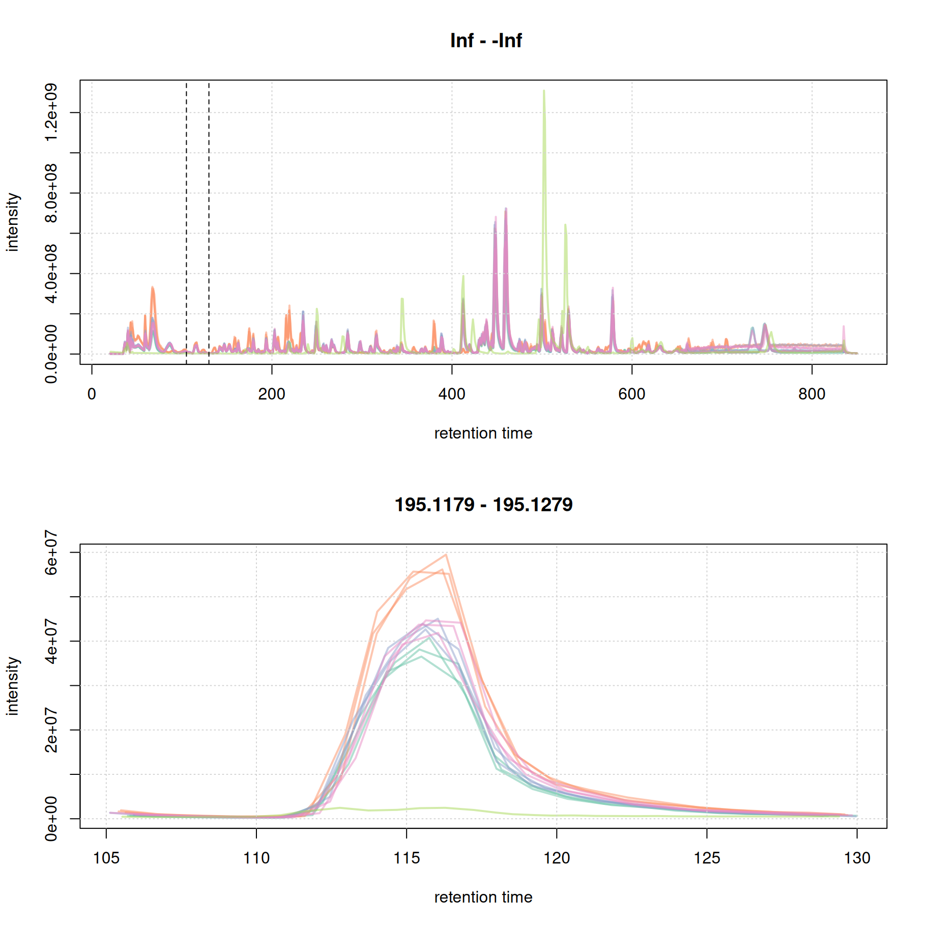
The width of this chromatographic peaks is about 8 seconds. We evaluate a second signal at the and of the chromatogram.
par(mfrow = c(2, 1))
plot(bpc, col = paste0(col_sample, 80), lwd = 2)
grid()

#' identify a region to extract
rtr_2 <- c(720, 770)
abline(v = rtr_2, lty = 2)

#' identify the m/z with the largest intensity in that region:
#' - restrict to MS1 data
#' - filter the MS data by retention time
#' - extract the MS data as a data.frame
tmp <- spectra(mse) |>
    filterMsLevel(1L) |>
    filterRt(rtr_2) |>
    longForm(columns = c("mz", "intensity"))

#' define a m/z range around the m/z with largest intensity
mzr_2 <- tmp$mz[which.max(tmp$intensity)] + c(-0.005, 0.005)

#' extract an EIC for that RT and m/z region
eic_2 <- chromatogram(mse, rt = rtr_2, mz = mzr_2)
plot(eic_2, col = paste0(col_sample, 80), lwd = 2)
grid()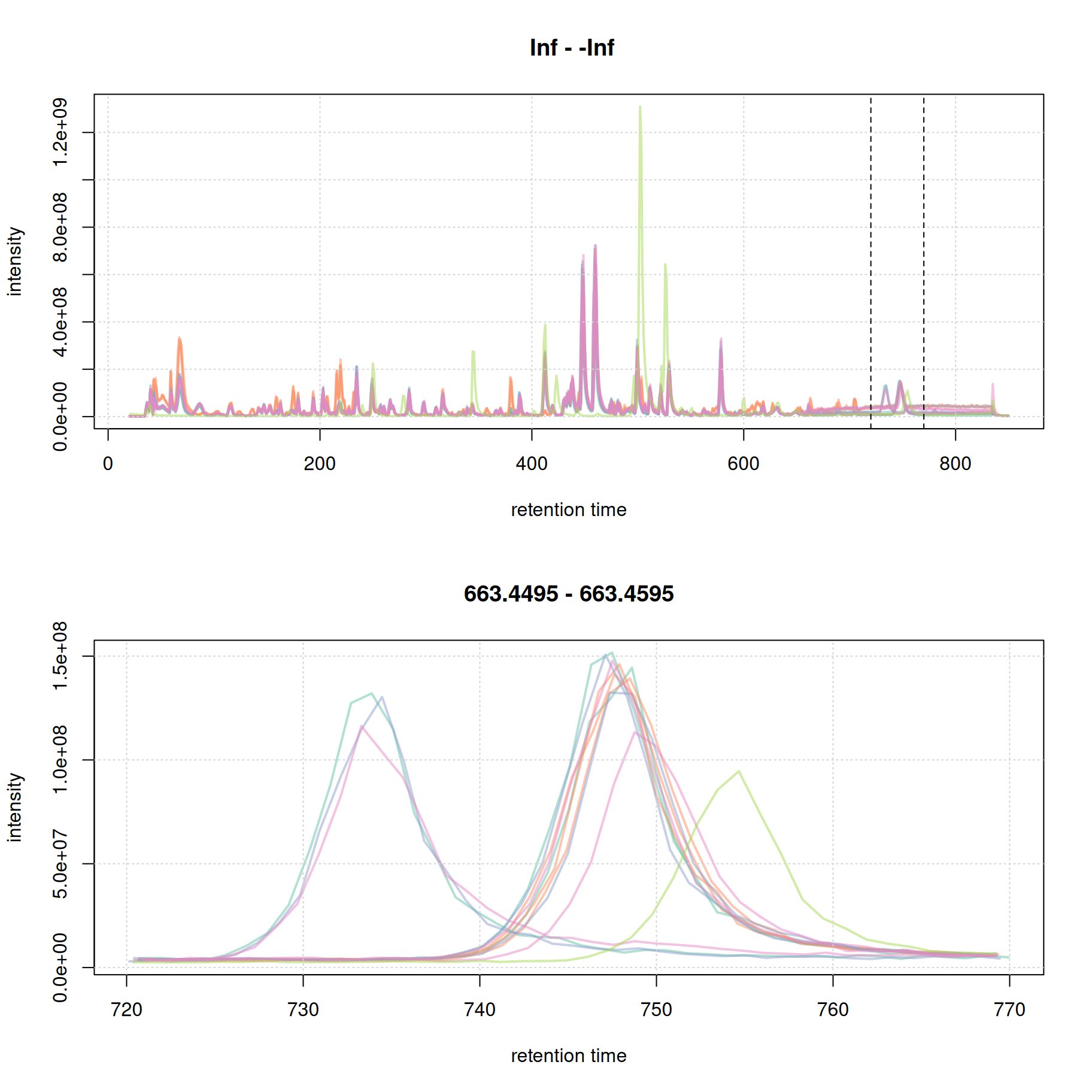
The width of the chromatographic peaks for that m/z slice seem to be around 15 seconds. Also, there seems to be a considerable shift in retention times between the samples.
Based on these two example signals we define the peakdwidth parameter for the present data set to be between and 5 and 20 seconds. For a real data analysis it is suggested to evaluate more signals, also eventually of internal standards or ions of compounds that are expected to be present in the sample.
A second potentially data set-specific parameter of the centWave algorithm is ppm. It defines the maximum allowed deviation in m/z dimension of mass peaks in consecutive spectra considered to represent signal from the same ion. To illustrate this we below subset the full MS data from the first data file to the m/z and retention time range defined above and plot the individual mass peaks.
ℹ️ Details on the
ppmcentWave parameterThe
ppmparameter defines the expected (or observed) m/z deviation of mass peaks representing signal from the same compound/ion in consecutive spectra. This scattering of mass peak’s m/z values can depend on the centroiding algorithm used or the precision of the MS instrument. In addition, on TOF instruments, the scattering can depend on the intensity of the signal, with higher variation observed for low intensity peaks and increasing stability with higher signal.
mse[1L] |>
    filterSpectra(filterMsLevel, 1L) |>
    filterSpectra(filterRt, rt = rtr_1) |>
    filterSpectra(filterMzRange, mz = mzr_1) |>
    plot()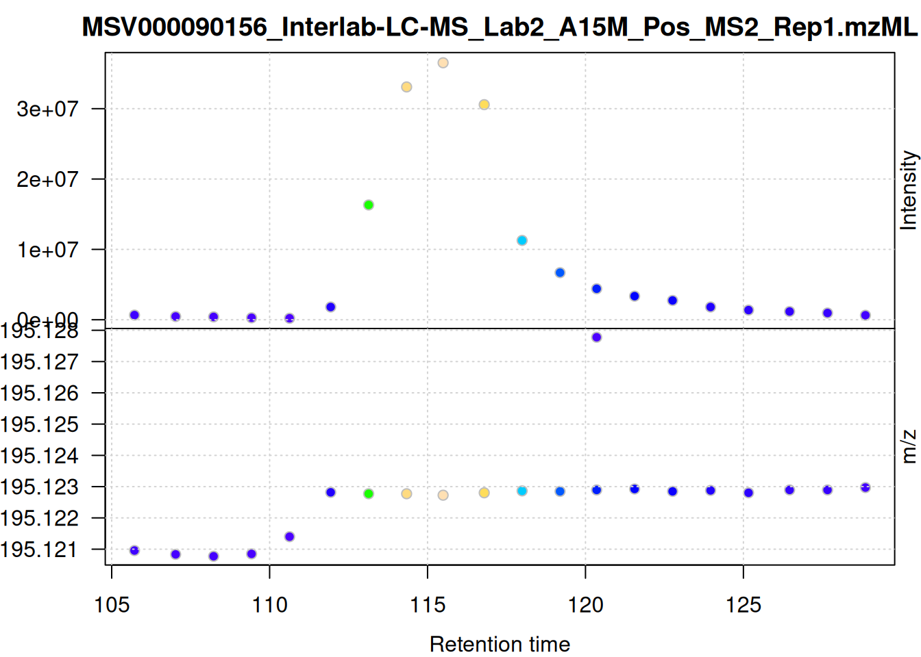
The individual mass peaks are shown in the lower panel in the plot above. For the present ion, the m/z values show a very low variance.
We evaluate the signal also for the second m/z - retention time window defined above.
mse[1L] |>
    filterSpectra(filterMsLevel, 1L) |>
    filterSpectra(filterRt, rt = rtr_2) |>
    filterSpectra(filterMzRange, mz = mzr_2) |>
    plot()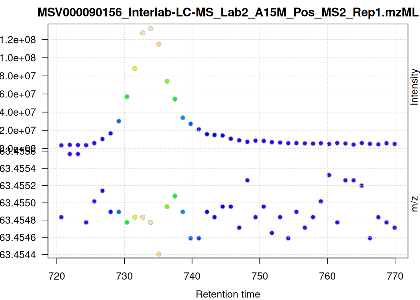
The scattering of m/z values looks larger, but is still below 0.001 Da. We nevertheless use a ppm = 20 for the present data set - as we do not assume that ions from different compounds elute at the same time with a difference in ppm lower than 20.
Below we define the settings for centWave and perform the chromatographic peak detection on the full data set. Note that it can also be helpful to test the different settings by performing peak detection on extracted ion chromatograms as described in Metabonaut. Parameter chunkSize defines the number of data files from which MS data should be loaded at a time. This parameter thus has an influence on the memory usage of the analysis.
#' configure and perform chromatographic peak detection
cwp <- CentWaveParam(
    ppm = 20,
    peakwidth = c(5, 20),
    snthresh = 8,
    integrate = 2,
    mzdiff = 0.001
)
mse <- findChromPeaks(mse, param = cwp, chunkSize = 4L)
In most cases it is also advisable to perform a peak postprocessing to remove artifacts of the centWave peak detection (e.g. overlapping or split peaks). Below we perform such peak refinement which will merge partially or completely overlapping chromatographic peak, or those that are less than 2 seconds apart from each other, if the intensity below both apexes is lower than a certain proportion of the apex intensity of the lower intensity peak.
#' configure and perform *peak refinement*
mnpp <- MergeNeighboringPeaksParam(
    expandRt = 1,
    expandMz = 0,
    ppm = 0,
    minProp = 0.75)
mse <- refineChromPeaks(mse, mnpp, chunkSize = 4L)
We next compare the number of identified peaks per sample as well as their m/z and retention time widths.
#' split the detected chrom peaks per sample
pk_list <- split.data.frame(
    chromPeaks(mse, columns = c("mzmin", "mzmax", "rtmin", "rtmax")),
    chromPeaks(mse, columns = "sample")[, "sample"])
#' calculate mz and rt widths
pk_list <- lapply(pk_list, function(z) {
    cbind(z, mz_width = z[, "mzmax"] - z[, "mzmin"],
          mz_width_ppm = (z[, "mzmax"] - z[, "mzmin"]) * 1e6 / z[, "mzmax"],
          rt_width = z[, "rtmax"] - z[, "rtmin"])
})

#' plot the information
par(mfrow = c(3, 1), mar = c(0, 4.3, 1.5, 0.1))
barplot(unlist(lapply(pk_list, nrow)),
     col = col_sample,
     ylab = "peak count", main = "Peak detection summary, mse", xaxt = "n")
grid()
legend("top", horiz = TRUE, col = col, pch = 15,
       legend = names(col))
par(mar = c(0, 4.3, 0, 0.1))
vioplot(lapply(pk_list, function(z) z[, "mz_width_ppm"]), outline = FALSE,
        ylab = "m/z width [ppm]", xaxt = "n", line = 3,
        col = col_sample)
grid()
vioplot(lapply(pk_list, function(z) z[, "rt_width"]),
        ylab = "rt width [s]", col = col_sample, line = 3)
grid()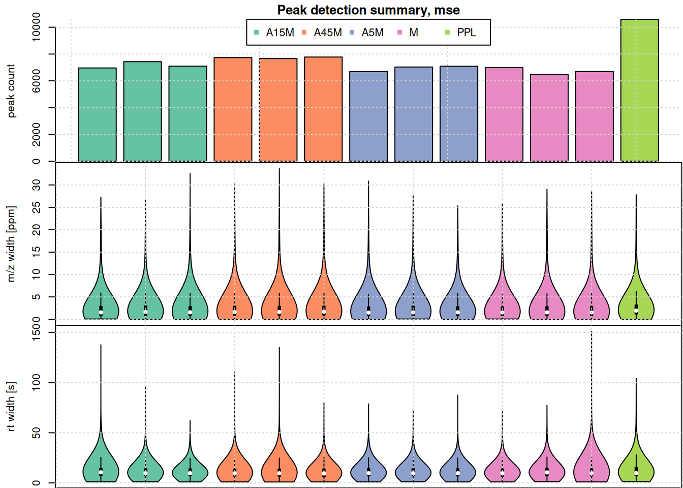
The highest number of peaks was detected in the PPL sample. Apart from that sample, the numbers of detected peaks is comparable in the data set. Also the m/z width and the retention time widths. As expected, most of the identified chromatographic peaks are about 10 seconds wide. Also, their m/z width is below 10 ppm for most peaks, but some show also a larger m/z widths.
We also evaluate the peak detection results on the two example m/z - retention time regions. Identified chromatographic peaks will be colored according to the sample group.
eic_1 <- chromatogram(mse, mz = mzr_1, rt = rtr_1)

#' define a color for each chromatographic peak
col_peak <- col_sample[chromPeaks(eic_1)[, "sample"]]
plot(eic_1, col = paste0(col_sample, 80),
     peakBg = paste0(col_peak, 10),
     peakCol = paste0(col_peak, 80))
grid()
legend("topright", col = col, lty = 1,
       legend = names(col))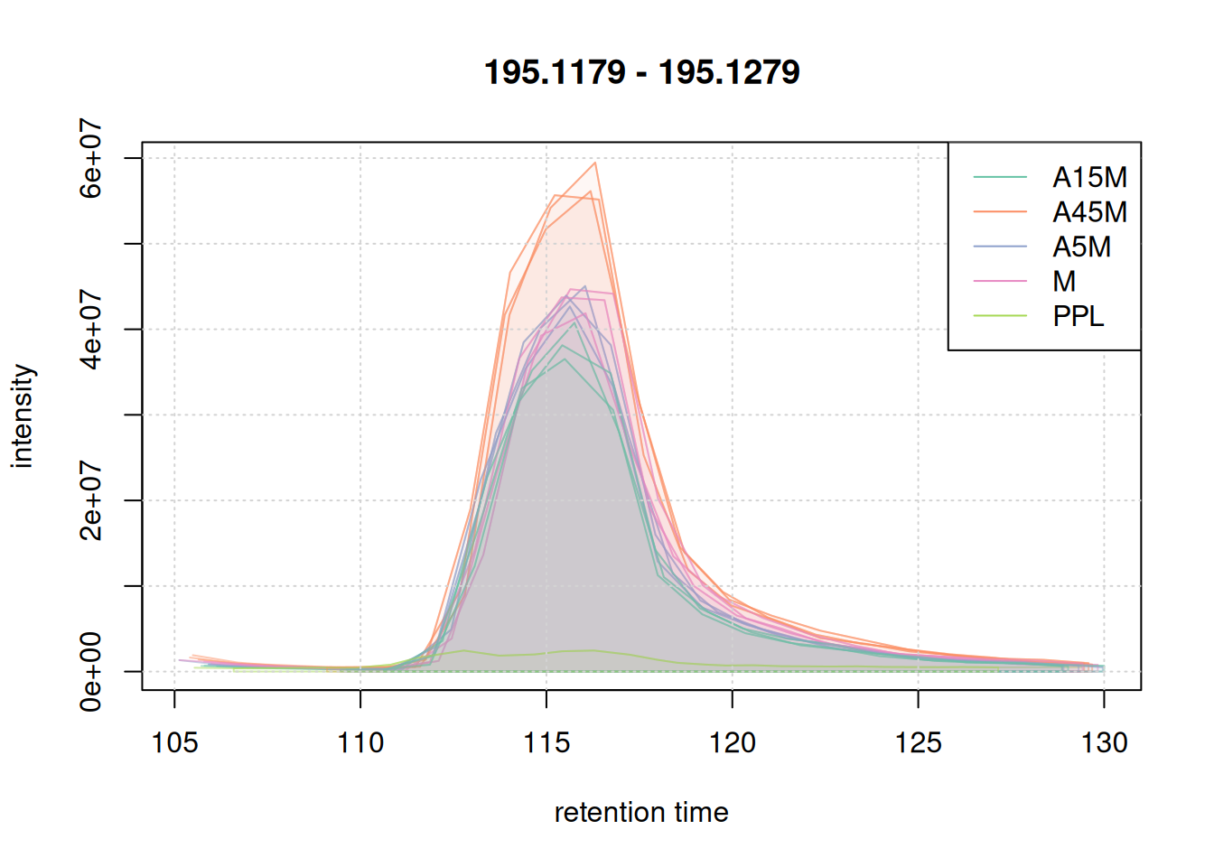
eic_2 <- chromatogram(mse, mz = mzr_2, rt = rtr_2)

#' define a color for each chromatographic peak
col_peak <- col_sample[chromPeaks(eic_2)[, "sample"]]
plot(eic_2, col = paste0(col_sample, 80),
     peakBg = paste0(col_peak, 10),
     peakCol = paste0(col_peak, 80))
grid()
legend("topright", col = col, lty = 1,
       legend = names(col))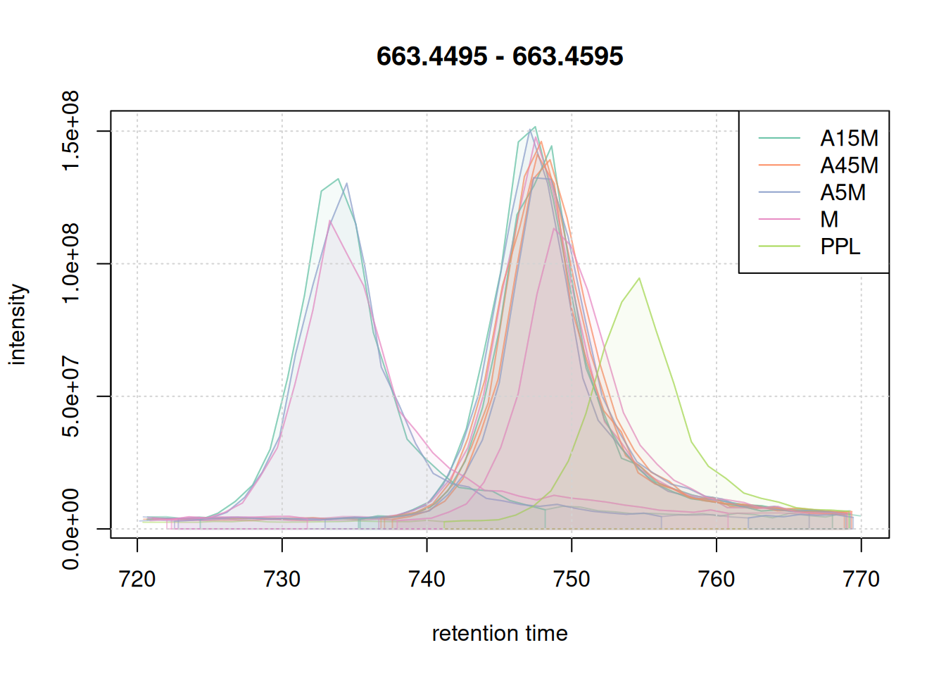
Retention time alignment
The aim of the retention time alignment step is to reduce differences observed in the elution time of compounds between different LC-MS runs. A variety of methods for this have been proposed and some are also implemented in xcms. We use the most straight forward approach that aligns chromatographic runs based on retention times of anchor peaks, i.e., compounds present in most of the samples of an experiment. To define these anchor peaks we must however perform an initial correspondence analysis and group chromatographic peaks with similar m/z and retention time across samples.
We use the peak density correspondence method which groups chromatographic peaks into an LC-MS feature, if their m/z difference is smaller than binSize (+ ppm of the m/z), the retention time of their apex is within one peak of the peak density curve (which smoothness can be configured with parameter bw) and a chromatographic peak is present in at least minFraction of at least one of the sample groups defined with sampleGroups. For the initial correspondence we apply more relaxed settings and consider all samples to be in the same sample group (since we want to define anchor peaks that are present in most samples).
ℹ️ Details on
PeakDensityParamsettingsThe peak density correspondence method can be configured using the
PeakDensityParam. For an initial correspondence used for retention time alignment more relaxed settings can be used, also putting all samples into the same sample group. The important parameters arebwandbinSize. The former defines the tolerance of retention time similarity, the latter the similarity of m/z values for chromatographic peaks from different samples to be considered to represent signal from ions of the same compound. SettingbinSizeis straight forward - it depends on the resolution of the instrument and the expected similarity of m/z values for the same ion. We set it to a value ofbinSize = 0.01, hence all chromatographic peaks with a difference in m/z smaller than 0.01 would be evaluated. Thebwparameter is a bit more difficult to define. It should be defined based on observed data in the experiment, ideally, on EICs of closely eluting compounds with the same m/z. In our example we use the second example m/z - retention time range, because it seemed to contain signal from the same compound, but with quite large shifts between data files. We below simulate a correspondence analysis on this EIC. Other parameters defined areminFraction, which defines the minimum required proportion of samples of one of the sample groups defined with parametersampleGroupsin which a chromatographic peak is present, andppmwhich, together withbinSizedefines the maximal accepted difference in chromatographic peaks’ m/z values to consider them for grouping.
pdp <- PeakDensityParam(
    sampleGroups = rep(1, length(mse)),
    bw = 2,
    minFraction = 0.2,
    binSize = 0.01,
    ppm = 10)

col_peak <- col_sample[chromPeaks(eic_2)[, "sample"]]
plotChromPeakDensity(eic_2, param = pdp, col = col_sample, peakCol = col_peak,
                     peakBg = paste0(col_peak, 40))
grid()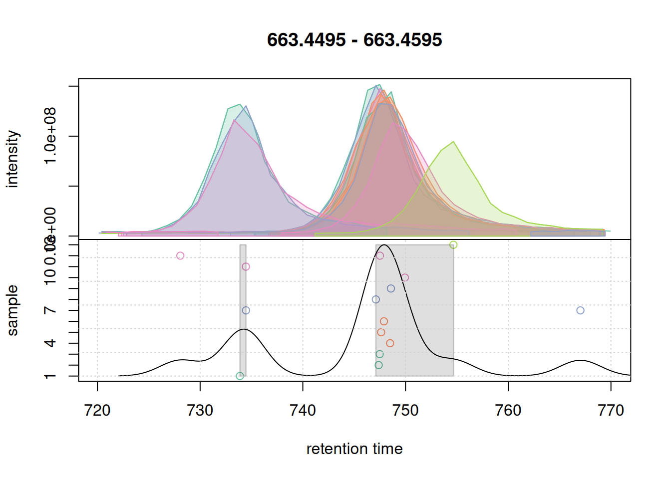
The upper panel of this plot shows the EIC, the lower panel the data considered for correspondence: it shows the retention time of the apex positions of all chromatographic peaks in that m/z slice on the x-axis against the sample in which the chromatographic peak was detected on the y-axis. The black solid line represents the peak density estimate, calculated based on the retention times of the chromatographic peaks and parameter bw with larger values of bw resulting in more smooth curves.
With the used settings, in particular parameter bw, the present chromatographic peaks would be split into two separate LC-MS features (indicated with a grey rectangle in the lower panel). Assuming that all peaks in that region represent signal from ions of the same compound, we however want to group them into the same feature. We hence next increase the bw parameter and simulate the correspondence with these updated settings.
pdp@bw <- 5
plotChromPeakDensity(eic_2, param = pdp, col = col_sample, peakCol = col_peak,
                     peakBg = paste0(col_peak, 40))
grid()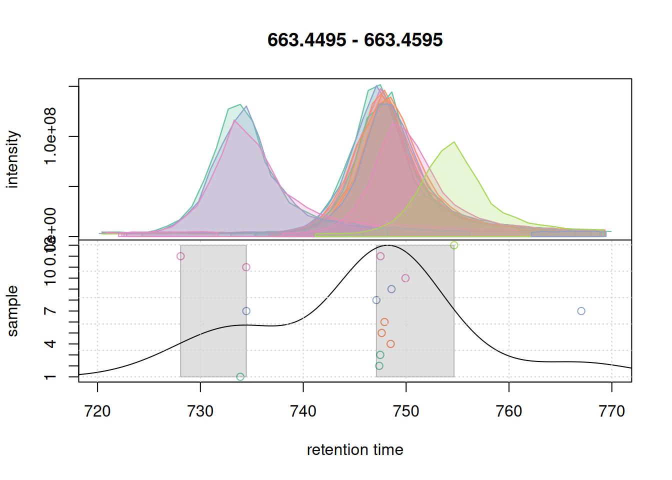
bw = 5.
Changing bw to 5 changed the density curve, but we still defined two separate features. We thus increase below bw to 7.
pdp@bw <- 7
plotChromPeakDensity(eic_2, param = pdp, col = col_sample, peakCol = col_peak,
                     peakBg = paste0(col_peak, 40))
grid()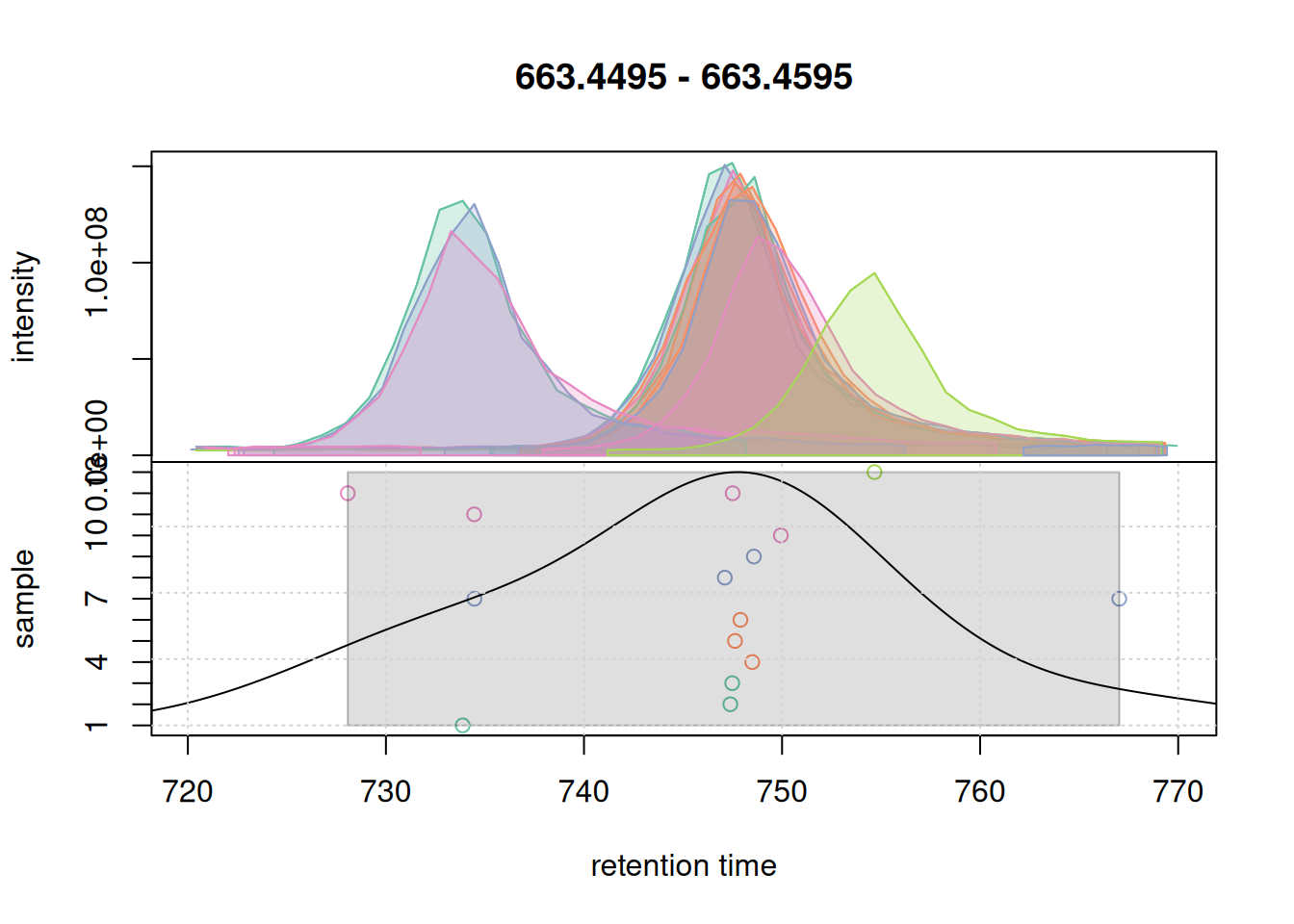
bw = 7.
With a bw = 7 a single feature was defined. We use these parameter for the initial correspondence analysis on the full data set.
#' perform initial correspondence analysis to group chromatographic peaks
mse <- groupChromPeaks(mse, param = pdp)
For the retention time alignment we use the before mentioned peak groups method that aligns LC runs by minimizing retention time differences of so called anchor peaks. This alignment method is very robust and also flexible, allowing for example to align samples based on within-experiment QC samples, or against external reference data or based on manually defined anchor peaks. See Metabonaut for examples and options. The method can be configured with PeakGroupsParam(). With minFraction = 0.9 we below define anchor peaks as those LC-MS features (defined by the initial correspondence analysis) for which a chromatographic peak was identified in 90% of the samples of the whole experiment. The observed retention time differences of these are used to model a curve along retention time dimension which is then used to align the retention times of all samples. The smoothness of this curve can be configured with parameter span (values between 0 and 1; values around 0.5 work in most cases).
#' configure and run retention time alignment
pgp <- PeakGroupsParam(
    minFraction = 0.90,
    span = 0.4)
mse <- adjustRtime(mse, param = pgp)
The effect of this alignment can be visualized with the plotAdjustedRtime() function. It plots the adjusted retention times of each sample on the x-axis against the difference between the adjusted and raw retention times on the y-axis as a solid line. Retention times of anchor peaks in each sample are indicated with individual data points. These should ideally be placed along the full retention time range of the experiment.
#' visualize alignment results
plotAdjustedRtime(mse, col = paste0(col_sample, 80),
                  peakGroupsPch = 21, lwd = 2)
grid()
legend("topleft", col = col, lty = 1,
       legend = names(col))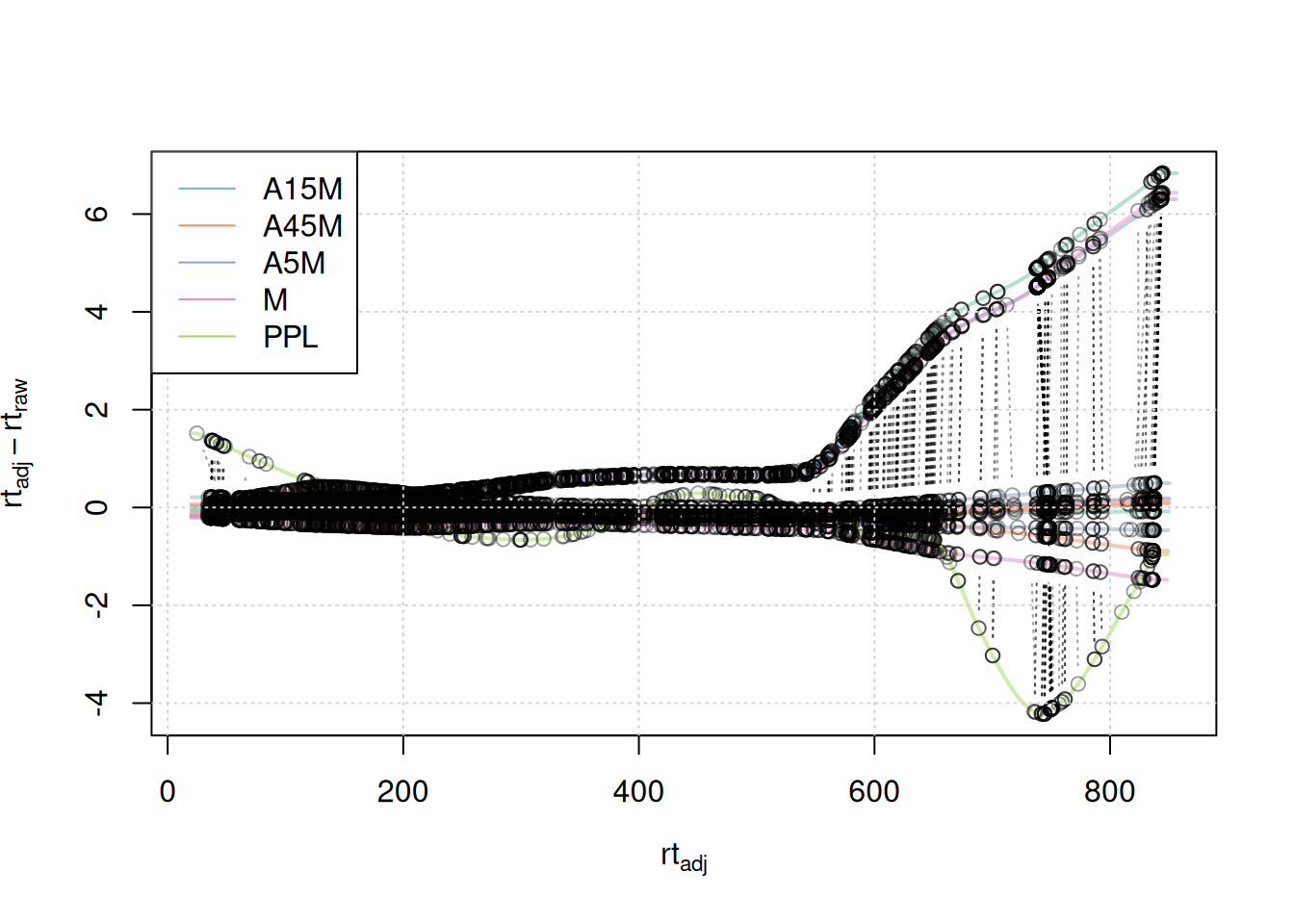
Anchor points span the full retention time range. Retention time adjustments for most samples were below 2-4 seconds, with the exception of 3 samples for which a considerably larger adjustment is present after 500 seconds, and the PPL sample with larger retention time differences after 650 seconds.
We next evaluate the alignment results based on the BPC before and after alignment.
#' create a BPC after adjustment; chromPeaks = "none" only creates the BPC
#' without extracting also identified chromatographic peaks.
bpc_adj <- chromatogram(mse, chromPeaks = "none", aggregationFun = "max")

par(mfrow = c(2, 1))
plot(bpc, col = paste0(col_sample, 80), main = "BPC, raw", lwd = 2)
grid()
legend("topright", col = col, legend = names(col), lty = 1, lwd = 2)
plot(bpc_adj, col = paste0(col_sample, 80), main = "BPC, adjusted", lwd = 2)
grid()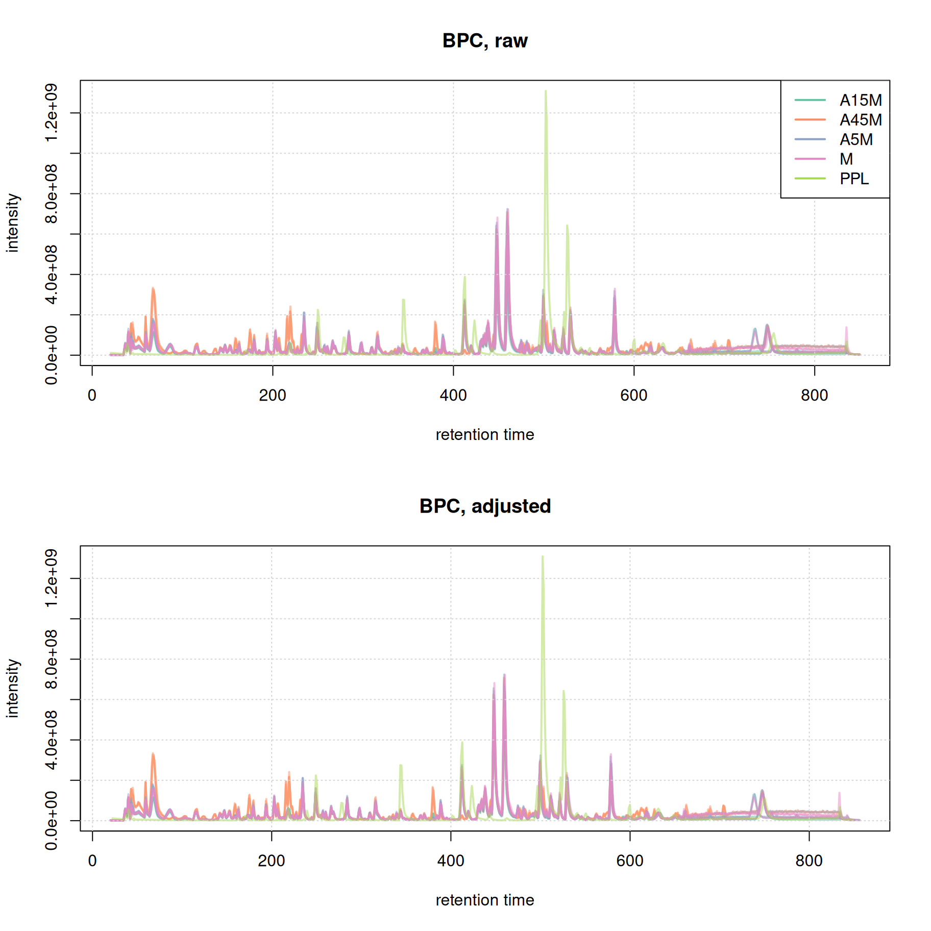
Misalignment of signal at the later stage of the chromatography seems to be reduced. We in addition evaluate the effect of retention time alignment on the two example EICs.
eic_1_adj <- chromatogram(mse, rt = rtr_1, mz = mzr_1, chromPeaks = "none")

par(mfrow = c(2, 1))
plot(eic_1, col = paste0(col_sample, 80), lwd = 2, peakType = "none")
grid()
legend("topright", col = col, legend = names(col), lty = 1, lwd = 2)
plot(eic_1_adj, col = paste0(col_sample, 80), lwd = 2)
grid()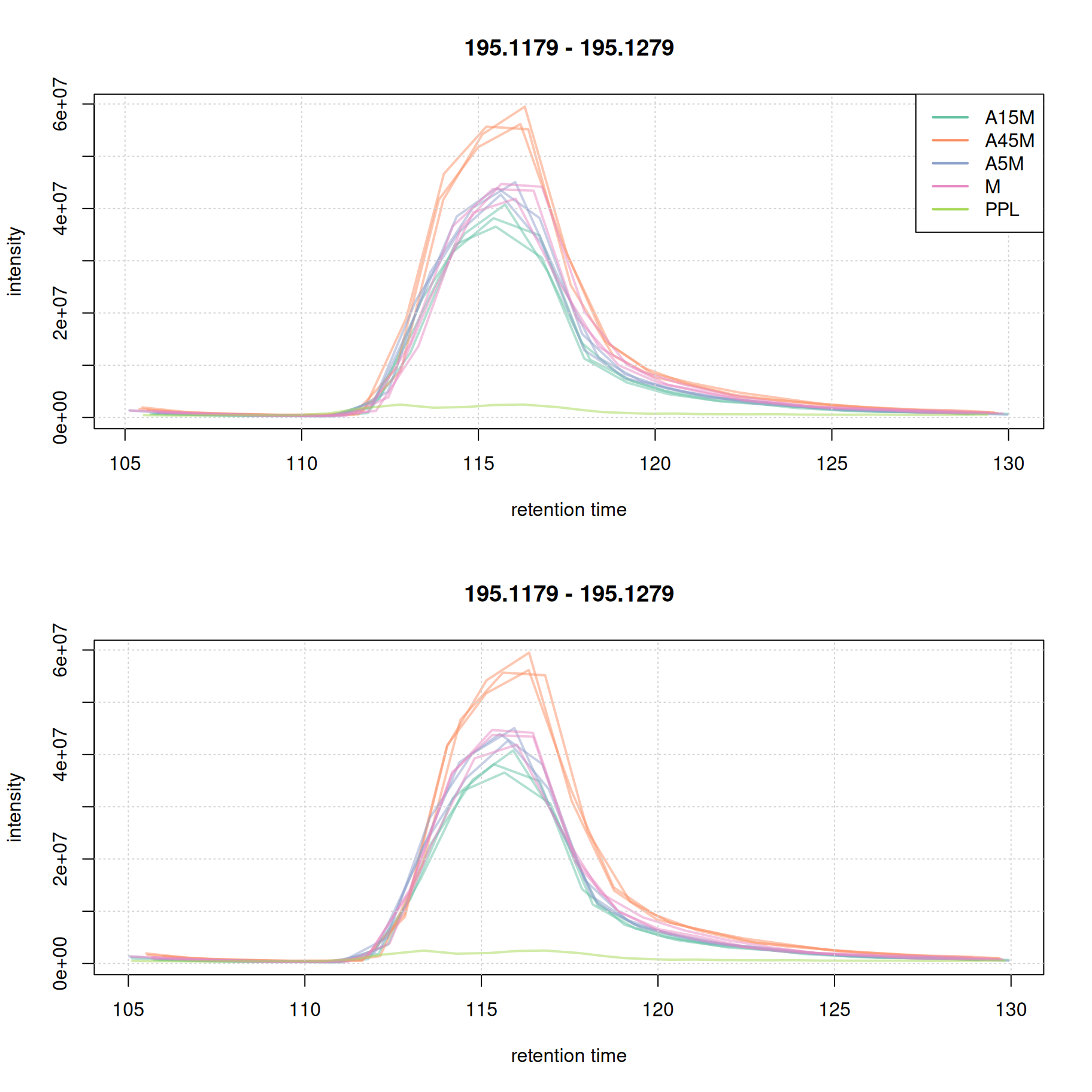
For this early retention time range already the raw signal was well aligned.
eic_2_adj <- chromatogram(mse, rt = rtr_2, mz = mzr_2, chromPeaks = "none")

par(mfrow = c(2, 1))
plot(eic_2, col = paste0(col_sample, 80), lwd = 2, peakType = "none")
grid()
legend("topright", col = col, legend = names(col), lty = 1, lwd = 2)
plot(eic_2_adj, col = paste0(col_sample, 80), lwd = 2)
grid()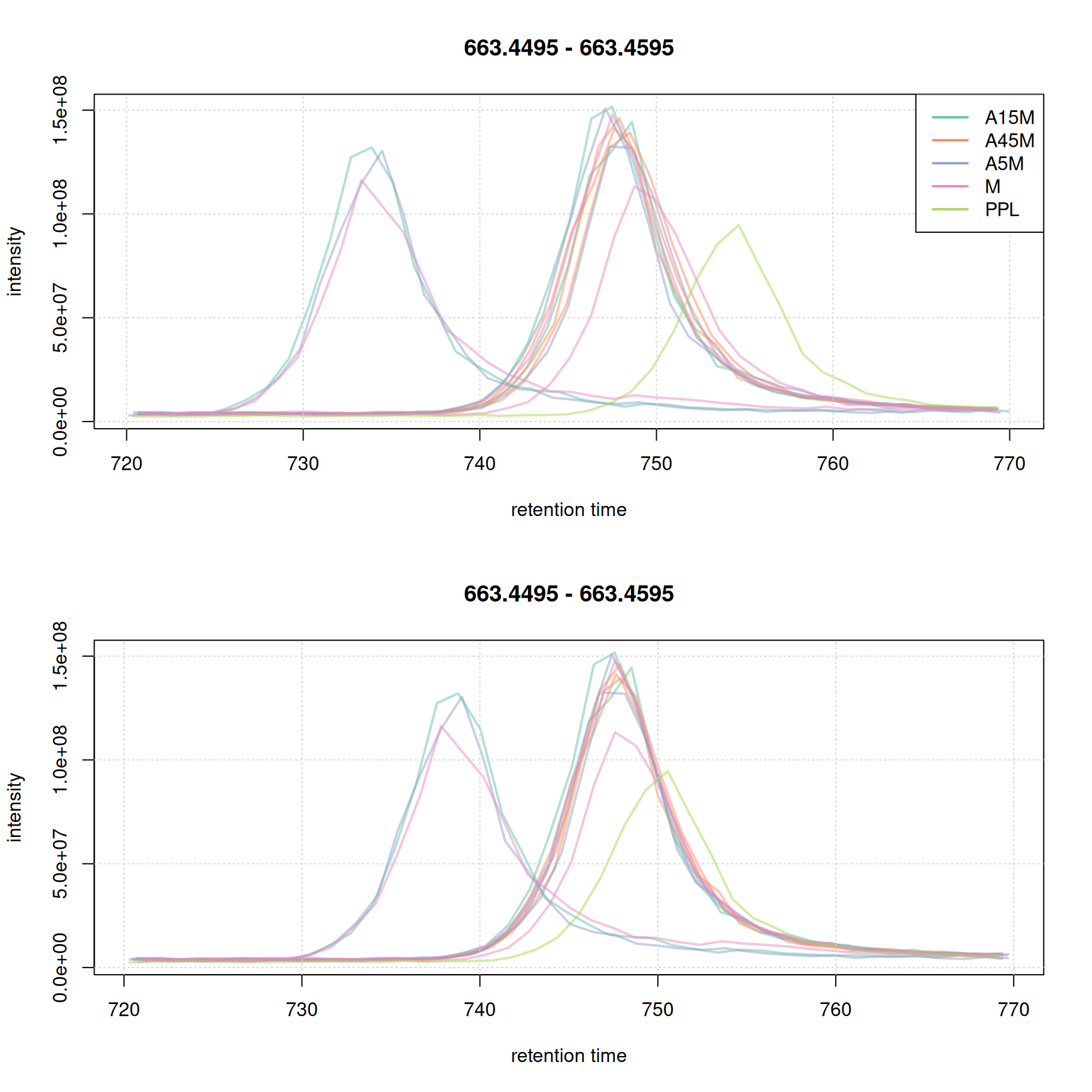
This later retention time range shows clear, and strong, differences in retention times of 4 samples. While the PPL sample could be aligned quite well using the above settings, 3 samples still show considerable shifts in retention times. We thus re-perform the alignment reducing the value for the span parameter to switch to a more local alignment of the samples. We below first undo the retention time alignment, re-perform the initial correspondence analysis and perform the alignment with the changed settings for parameter span.
#' remove retention time alignment results
mse <- dropAdjustedRtime(mse)
#' re-perform initial correspondence
mse <- groupChromPeaks(mse, param = pdp)
#' perform the alignment using updated settings
pgp <- PeakGroupsParam(
    minFraction = 0.90,
    span = 0.1)
mse <- adjustRtime(mse, param = pgp)
Evaluating the impact of changing this parameter.
#' visualize alignment results
plotAdjustedRtime(mse, col = paste0(col_sample, 80),
                  peakGroupsPch = 21, lwd = 2)
grid()
legend("topleft", col = col, lty = 1,
       legend = names(col))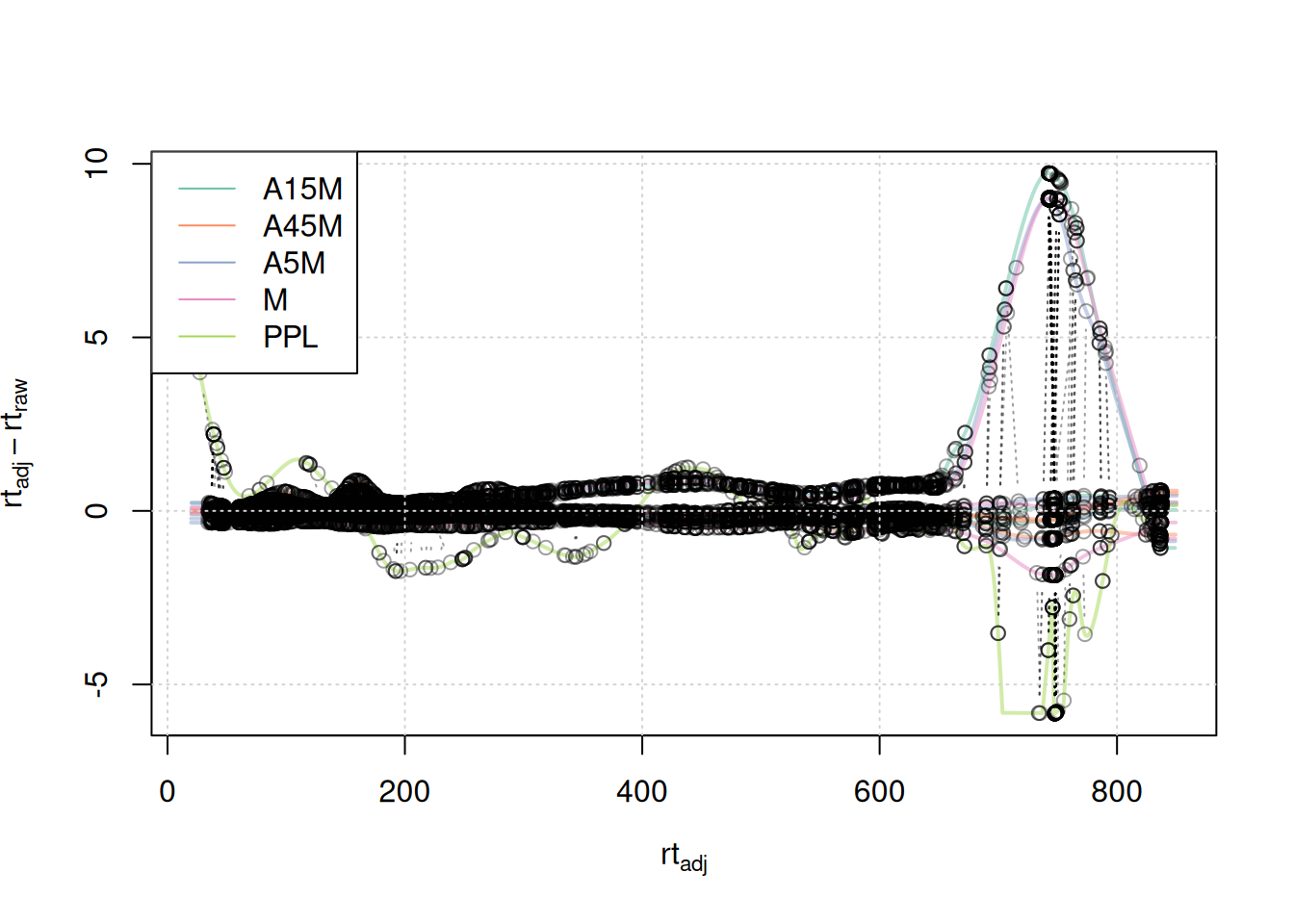
A stronger alignment can be observed for the retention time area from 750 to 800 seconds. The results for the first example EIC did not change.
eic_1_adj <- chromatogram(mse, rt = rtr_1, mz = mzr_1)

par(mfrow = c(2, 1))
#' Setting peakType = "none" prevents identified chromatographic peaks to be
#' indicated in the plot.
plot(eic_1, col = paste0(col_sample, 80), lwd = 2, peakType = "none")
grid()
legend("topright", col = col, legend = names(col), lty = 1, lwd = 2)
plot(eic_1_adj, col = paste0(col_sample, 80), lwd = 2, peakType = "none")
grid()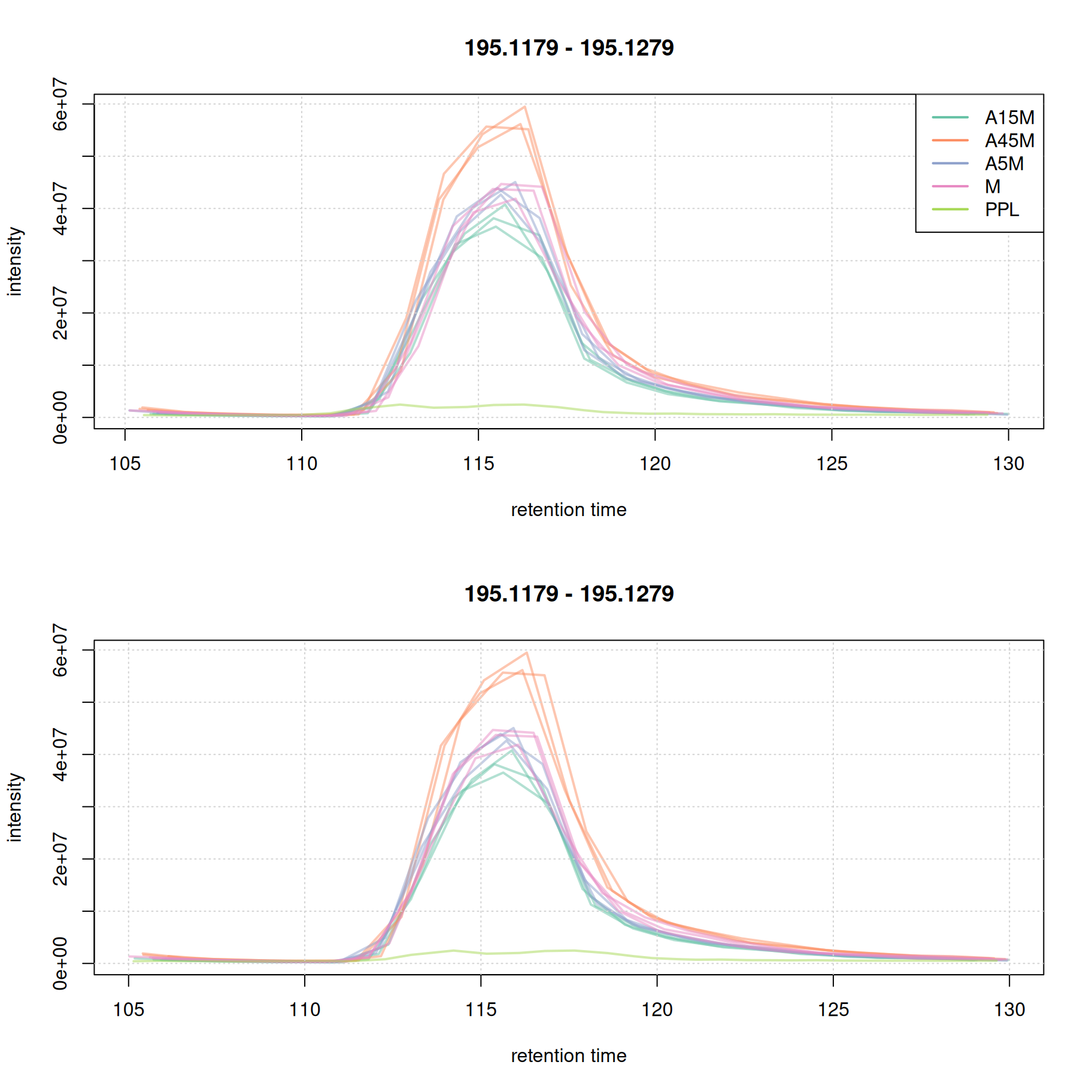
While for the second EIC the alignment improved.
eic_2_adj <- chromatogram(mse, rt = rtr_2, mz = mzr_2)

par(mfrow = c(2, 1))
plot(eic_2, col = paste0(col_sample, 80), lwd = 2, peakType = "none")
grid()
legend("topright", col = col, legend = names(col), lty = 1, lwd = 2)
plot(eic_2_adj, col = paste0(col_sample, 80), lwd = 2, peakType = "none")
grid()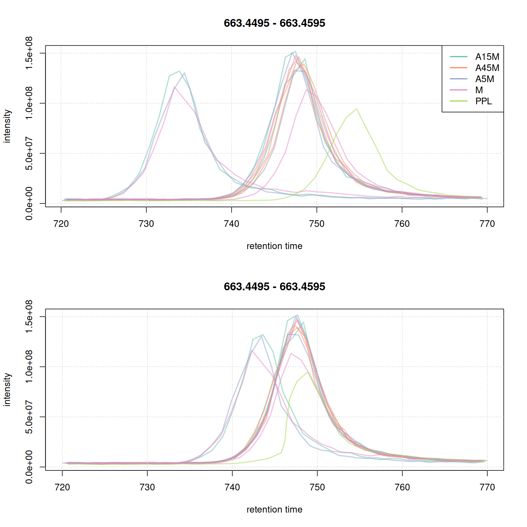
:information_source: note that in most cases it is not necessary that all samples are perfectly aligned. Some variation in retention time can be accounted for in the final correspondence analysis.
Correspondence analysis
The correspondence analysis groups chromatographic peaks from different samples, all assumed to represent signal from ions of the same compound, into LC-MS features. Signals are generally grouped together based on similarity of their m/z and retention times. We use the peak density method and, similarly to what we did in the previous section, we first evaluate the impact of different parameter settings on the expected results. Also, for the final correspondence we use the samples’ sample_name for parameter sampleGroup. Combined with setting minFraction = 0.67, an LC-MS feature is defined if a chromatographic peak is present in at least 67% of the replicates per sample (i.e., 2 out of 3).
#' configure the *peak density* correspondence method
pdp <- PeakDensityParam(
    sampleGroups = sampleData(mse)$sample_name,
    minFraction = 0.67,
    binSize = 0.01,
    ppm = 10,
    bw = 7)
We evaluate these settings, in particular the effect of bw on the first example EIC.
col_peak <- col_sample[chromPeaks(eic_1_adj)[, "sample"]]
plotChromPeakDensity(eic_1_adj, param = pdp, col = col_sample,
                     peakCol = col_peak, peakBg = paste0(col_peak, 40))
grid()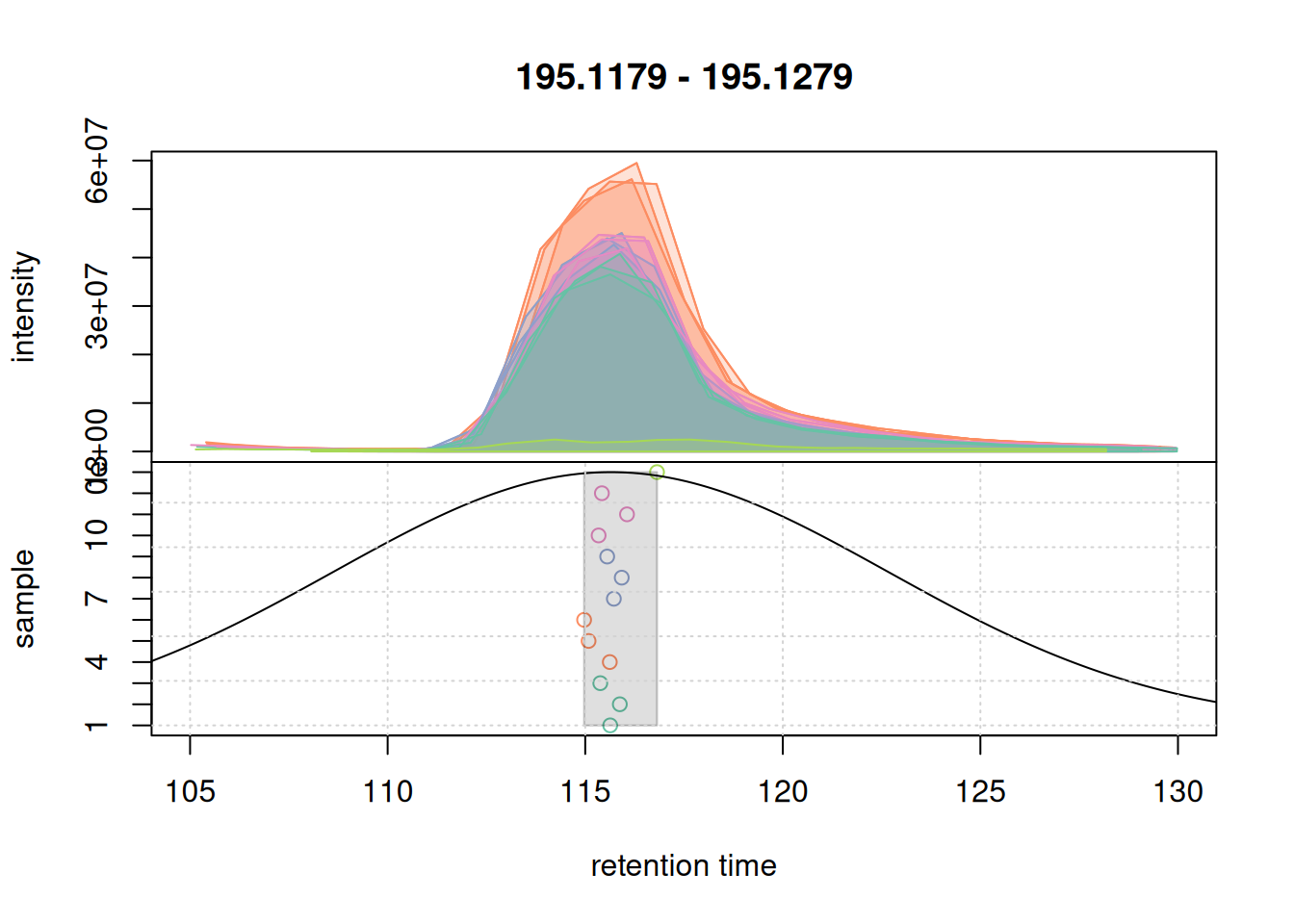
For that EIC the settings worked nicely. Simulating the correspondence for the second example EIC.
col_peak <- col_sample[chromPeaks(eic_2_adj)[, "sample"]]
plotChromPeakDensity(eic_2_adj, param = pdp, col = col_sample,
                     peakCol = col_peak, peakBg = paste0(col_peak, 40))
grid()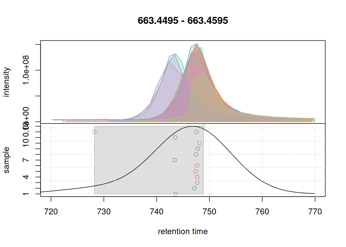
Also for the second EIC all chromatographic peaks got grouped into the same feature. Ideally, correspondence parameters should also be simulated on more complex signals, e.g. regions with co- or closely eluting compounds. We below expand the retention time window for the m/z slice of the first example EIC.
a <- chromatogram(mse, mz = mzr_1, rt = c(30, 150))

col_peak <- col_sample[chromPeaks(a)[, "sample"]]
plotChromPeakDensity(a, param = pdp, col = col_sample,
                     peakCol = col_peak, peakBg = paste0(col_peak, 40))
grid()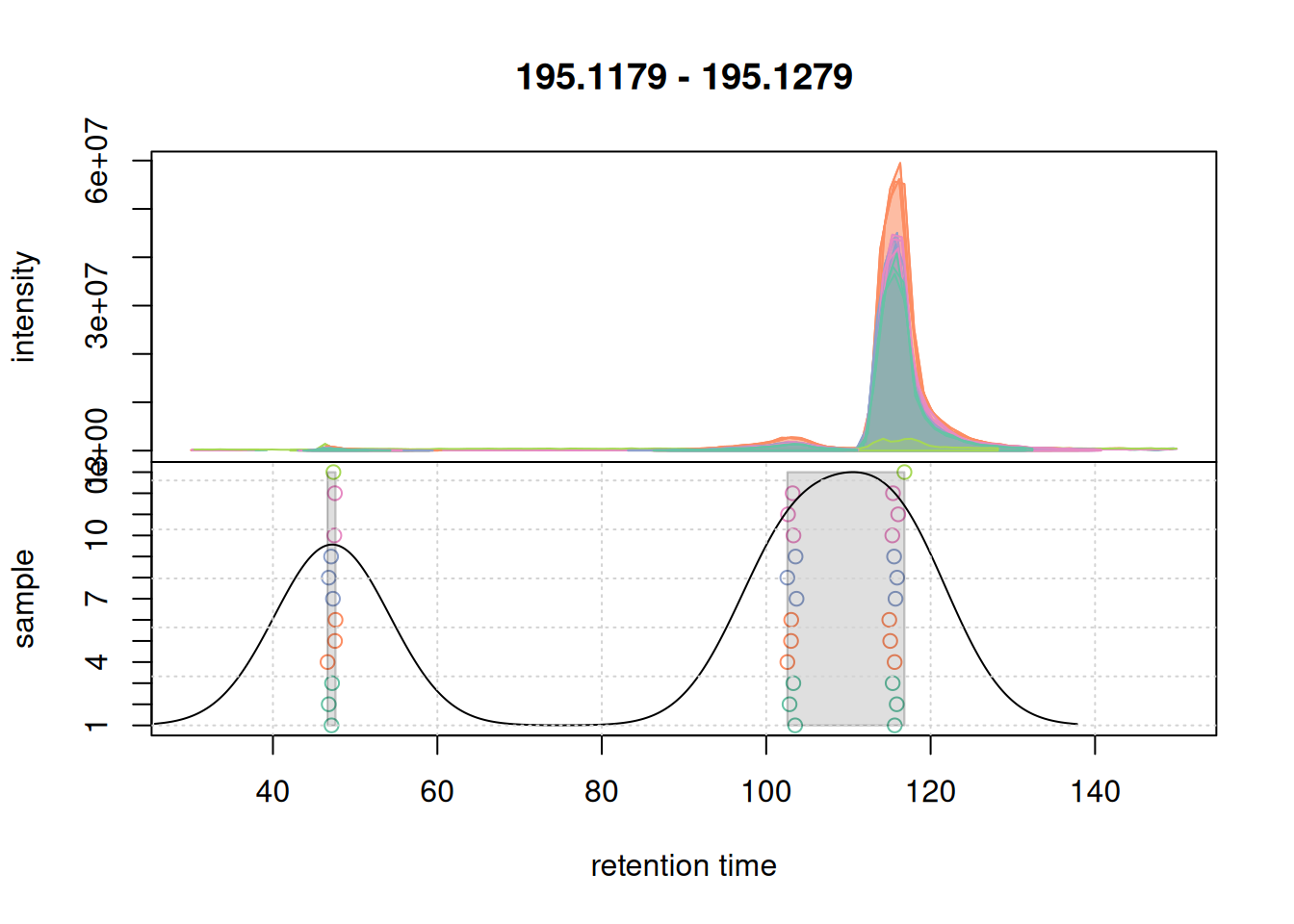
There seem to be signal from 3 different compounds in that m/z slice. Using the settings above, in particular with bw = 7 the apparently different chromatographic signals at about 105 and 115 seconds are grouped into the same LC-MS feature as indicated with the grey rectangle in the plot above. Unless we want that these signals are grouped together, we need to reduce the value of bw. Below we simulate a correspondence using bw = 3.
pdp@bw <- 3
plotChromPeakDensity(a, param = pdp, col = col_sample,
                     peakCol = col_peak, peakBg = paste0(col_peak, 40))
grid()
bw = 3 for the correspondence analysis.
With bw = 3 we successfully grouped the signals into 3 distinct features. We next evaluate whether with these updated setting we would still group the signal from the second example EIC into a single feature.
col_peak <- col_sample[chromPeaks(eic_2_adj)[, "sample"]]
plotChromPeakDensity(eic_2_adj, param = pdp, col = col_sample,
                     peakCol = col_peak, peakBg = paste0(col_peak, 40))
grid()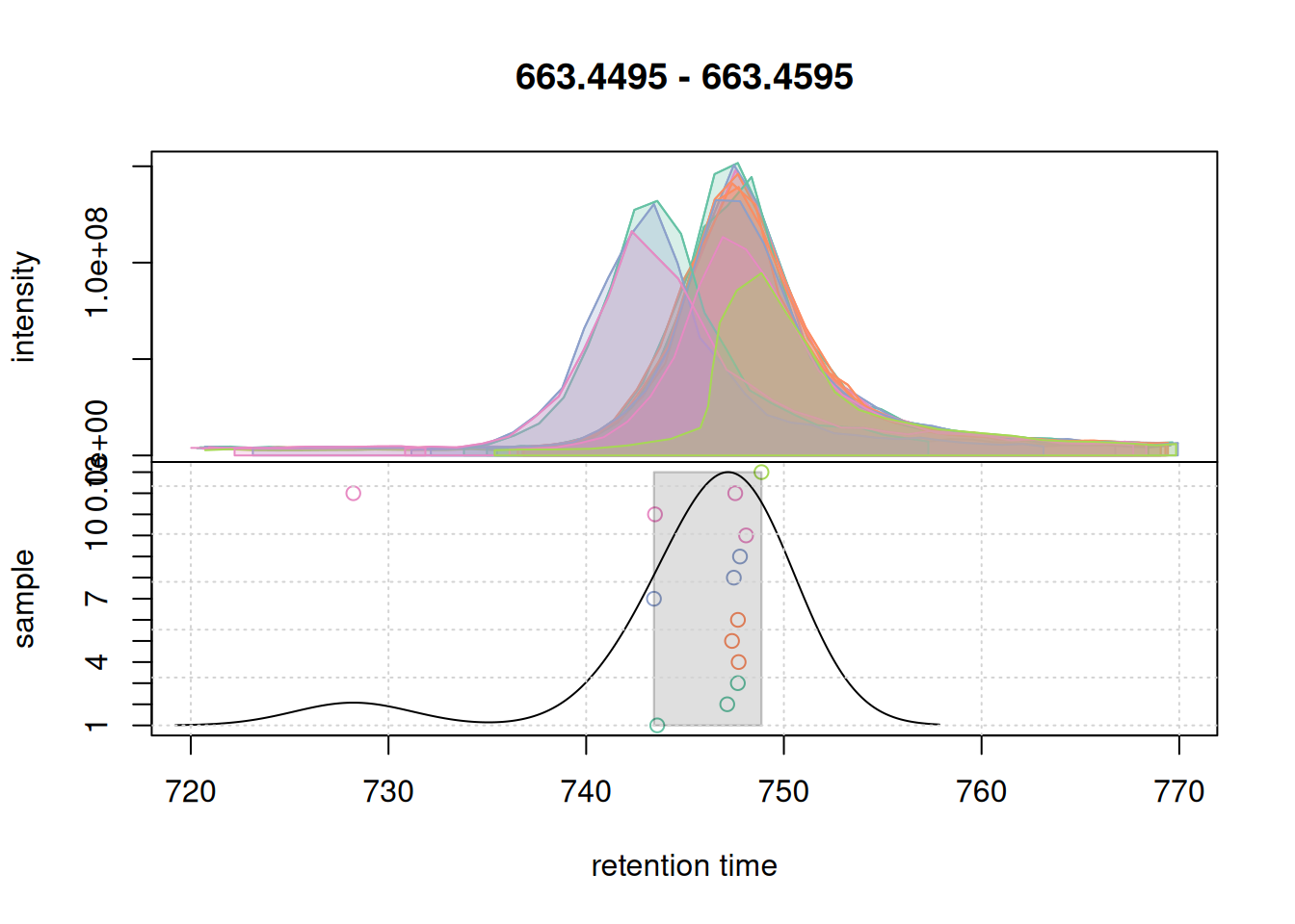
bw = 3 on correspondence results of the second example EIC.
All chromatographic peaks for this region were grouped into a single region. We thus proceed and use these settings for the correspondence analysis of the full data set.
#' perform correspondence analysis on the full data set
mse <- groupChromPeaks(mse, param = pdp)
It is advised to check the results again after correspondence analysis, also to evaluate the impact of the other settings like binSize and ppm and assure validity of the defined LC-MS features. Ideally, a larger number of EICs/features should be checked. We below extract the first example EIC again and evaluate the correspondence results for it. Here it is important to set simulate = FALSE to show the actual results.
eic_1 <- chromatogram(mse, rt = rtr_1, mz = mzr_1)

#' plot the actual correspondence results by setting `simulate = FALSE`
col_peak <- col_sample[chromPeaks(eic_1)[, "sample"]]
plotChromPeakDensity(eic_1, col = col_sample, peakCol = col_peak,
                     peakBg = paste0(col_peak, 40),
                     simulate = FALSE)
grid()
All chromatographic peaks were grouped into the same feature. The retention time ("rtmed") of the feature is indicated with a dashed vertical line. We next evaluate the results also on the second example EIC.
eic_2 <- chromatogram(mse, rt = rtr_2, mz = mzr_2)

#' plot the actual correspondence results by setting `simulate = FALSE`
col_peak <- col_sample[chromPeaks(eic_2)[, "sample"]]
plotChromPeakDensity(eic_2, col = col_sample, peakCol = col_peak,
                     peakBg = paste0(col_peak, 40),
                     simulate = FALSE)
grid()
Also for this retention time region, chromatographic peaks were grouped into a single feature. At last we evaluate the expanded retention time region of the m/z range of the first example EIC.
a <- chromatogram(mse, mz = mzr_1, rt = c(30, 150))

col_peak <- col_sample[chromPeaks(a)[, "sample"]]
plotChromPeakDensity(a, col = col_sample, peakCol = col_peak,
                     peakBg = paste0(col_peak, 40),
                     simulate = FALSE)
grid()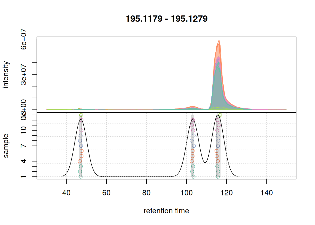
For this region, chromatographic peaks were grouped into 3 distinct features.
The results from the correspondence analysis can be extracted from the result object using the featureDefinitions() and featureValues() functions. The former returns the definition of the LC-MS features, i.e., their m/z and retention time, the latter the actual abundance estimates in the different samples. We below count the number of features that were defined by the correspondence analysis:
featureDefinitions(mse) |>
    nrow()
[1] 14808A quite large number of features was defined. This is mostly due to the setting for the minFraction parameter, which required a chromatographic peak to be detected in only 2 out of the 3 replicates for each individual sample to define, and combine them into, a feature.
We can now extract the abundance estimates of all features with the featureValues() function. Below we extract this data matrix and assign the unique sample name as column names (by default the MS data file name is used).
fvals <- featureValues(mse, method = "sum")
colnames(fvals) <- sampleData(mse)$sample_desc
head(fvals)
A15M_R1 A15M_R2 A15M_R3 A45M_R1 A45M_R2 A45M_R3 A5M_R1 A5M_R2 A5M_R3
FT00001 NA NA NA NA NA NA NA NA NA
FT00002 NA NA NA NA NA NA NA NA NA
FT00003 NA NA NA NA NA NA NA NA NA
FT00004 NA 3392535 NA 10258668 NA 9478585 5519297 NA NA
FT00005 NA NA NA 9521460 NA 6722026 2419544 NA NA
FT00006 NA NA NA 4874998 NA 5897690 3338828 NA NA
M_R1 M_R2 M_R3 PPL_R1
FT00001 NA NA NA 127518.4
FT00002 NA NA NA 201678.3
FT00003 NA NA NA 502676.9
FT00004 3684237 NA NA 6198111.3
FT00005 3405333 NA NA 2953772.8
FT00006 NA NA NA 6931111.8Columns in this abundance matrix are samples, rows features. For the present data set there are a large number of missing values. A missing value indicates failure to detect a chromatographic peak for the m/z - retention time region of a feature in a sample. This can have multiple reasons: the compound might simply not be present in the sample or the original signal is too noisy, to low in abundance, or does not fit the expected shape for the peak detection algorithm to identify a chromatographic peak.
Below we calculate and plot the number of missing values per sample.
#' determine the number of missing values per sample and plot them
nas <- apply(fvals, MARGIN = 2, function(z) sum(is.na(z)))

barplot(nas, main = "Number of missing values", col = col_sample)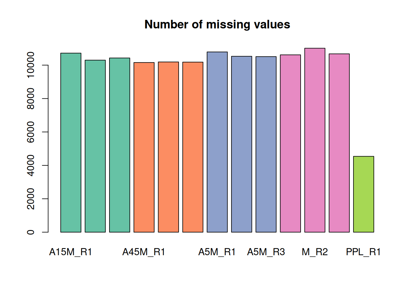
The lowest number of missing values is present in the PPL_R1 sample.
Gap-filling
To reduce the number of missing values and avoid data imputation we perform gap-filling: in samples with a missing value for a feature (i.e., in which no chromatographic peak was detected) we integrate all intensities measured within the m/z - retention time area of the feature. By default, this area is defined as the 25% to 75% quantile of the lower, respectively upper m/z (and retention time) boundary of all chromatographic peaks of a feature. As an example we calculate this area with the featureArea() function for the first 6 features:
featureArea(mse,
            mzmin = function(z) quantile(z, probs = 0.25, na.rm = TRUE),
            mzmax = function(z) quantile(z, probs = 0.75, na.rm = TRUE),
            rtmin = function(z) quantile(z, probs = 0.25, na.rm = TRUE),
            rtmax = function(z) quantile(z, probs = 0.75, na.rm = TRUE),
            features = rownames(featureDefinitions(mse))[1:4])
mzmin mzmax rtmin rtmax
FT00001 150.0268 150.0270 588.3672 594.2322
FT00002 150.0789 150.0791 166.7511 175.2998
FT00003 150.0912 150.0916 245.4199 254.4996
FT00004 150.1022 150.1030 812.2422 837.7419Thus, for gap-filling, missing values are replaced with the integrated signal measured by the MS instrument within these m/z - retention time boundaries.
We below perform the gap-filling on the full data set.
#' configure and perform gap-filling
cpap <- ChromPeakAreaParam(minMzWidthPpm = 10)
mse <- fillChromPeaks(mse, param = cpap, chunkSize = 4L)
We extract the feature values again and determine the number of missing values.
fvals <- featureValues(mse, method = "sum")
colnames(fvals) <- sampleData(mse)$sample_desc
head(fvals)
A15M_R1 A15M_R2 A15M_R3 A45M_R1 A45M_R2 A45M_R3 A5M_R1
FT00001 NA NA NA NA NA NA NA
FT00002 NA NA NA NA NA NA NA
FT00003 725629.5 395193.8 609652.6 709672 712048.4 325696.1 582689.3
FT00004 6667479.8 3392535.0 10874295.1 10258668 9681633.2 9478584.9 5519297.2
FT00005 4424076.9 5594730.1 8961144.0 9521460 7483711.7 6722025.8 2419544.4
FT00006 5058937.4 6075048.7 8164059.6 4874998 7531471.2 5897690.0 3338828.4
A5M_R2 A5M_R3 M_R1 M_R2 M_R3 PPL_R1
FT00001 NA NA 56655.1 NA NA 127518.4
FT00002 NA NA NA NA NA 201678.3
FT00003 737115.2 653138 470292.9 357432 463980.4 502676.9
FT00004 10336613.6 6591140 3684237.3 6720029 8384267.6 6198111.3
FT00005 10403154.3 5371937 3405332.8 5232400 8119441.8 2953772.8
FT00006 7827918.6 6753662 5360799.4 4505007 7968544.6 6931111.8
#' determine the number of missing values per sample and plot them
nas <- apply(fvals, MARGIN = 2, function(z) sum(is.na(z)))

barplot(nas, main = "Number of missing values", col = col_sample)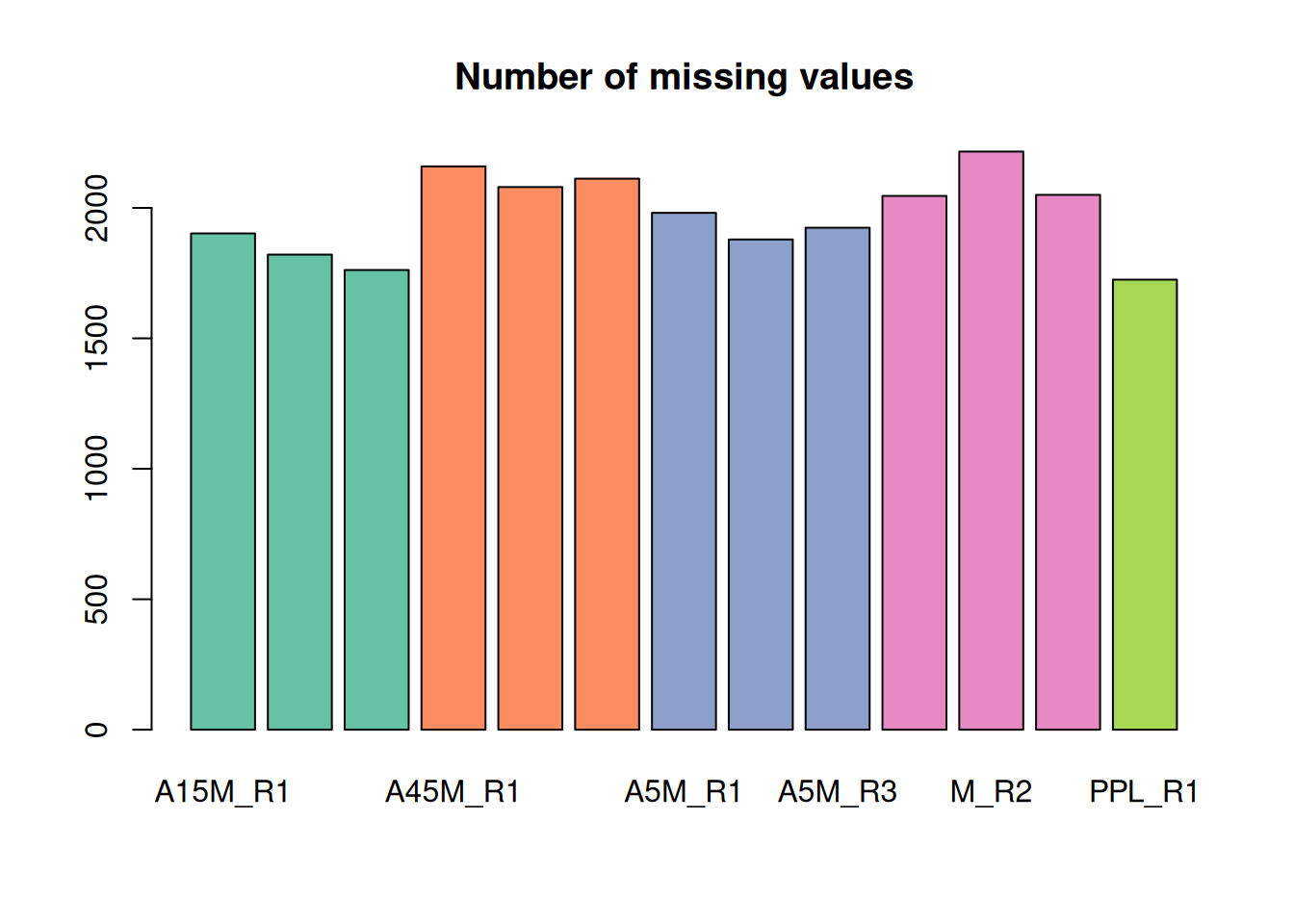
A considerable amount of values could thus be rescued.
Extract fragment spectra for LC-MS features
After preprocessing, we next identify and extract the MS2 spectra for the defined LC-MS features. We use the featureSpectra() method, that identifies for each of the features’ chromatographic peaks MS2 spectra (within the same sample!) with their retention time and precursor m/z within the retention time and m/z range of the chromatographic peak.
#' identify MS2 spectra for features
ms2 <- featureSpectra(mse)
ms2
MSn data (Spectra) with 21917 spectra in a MsBackendMassIVE backend:
msLevel rtime scanIndex
<integer> <numeric> <integer>
1 2 169.361 834
2 2 169.909 837
3 2 170.225 844
4 2 169.786 845
5 2 169.721 844
... ... ... ...
21913 2 748.486 3747
21914 2 747.600 3748
21915 2 744.174 3679
21916 2 748.223 3744
21917 2 749.801 3791
... 43 more variables/columns.
file(s):
MSV000090156_Interlab-LC-MS_Lab2_A15M_Pos_MS2_Rep2.mzML
MSV000090156_Interlab-LC-MS_Lab2_A15M_Pos_MS2_Rep3.mzML
MSV000090156_Interlab-LC-MS_Lab2_A45M_Pos_MS2_Rep1.mzML
... 10 more files
Processing:
Filter: select retention time [20..850] on MS level(s) [Thu Jul 2 09:29:56 2026]
Filter: select MS level(s) 2 [Thu Jul 2 09:36:18 2026]
Filter: select MS level(s) 2 [Thu Jul 2 09:36:21 2026]
...3 more processings. Use 'processingLog' to list all. We can have multiple, or no, MS2 spectra per feature:
#' count the number of MS2 spectra per feature
ms2_count <- table(ms2$feature_id)

#' the number of LC-MS features with at least one MS2 spectrum:
length(ms2_count)
[1] 3091
#' the average number of MS2 spectra per feature:
mean(ms2_count)
[1] 7.090586We next inspect some of the identified MS2 spectra.
#' select MS2 spectra for the first feature
a <- ms2[ms2$feature_id == ms2$feature_id[1]]

#' plot the spectra
plotSpectra(a)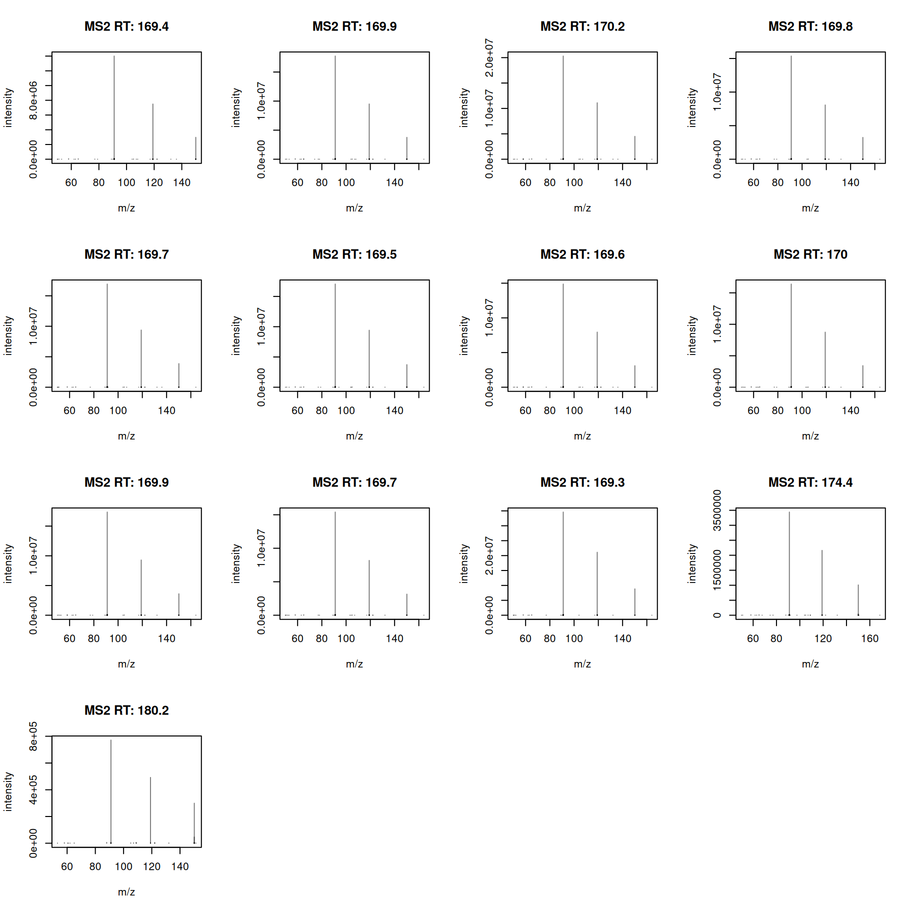
All MS2 spectra look similar - we next calculate also a pairwise similarity between them and visualize the results as a heatmap.
#' calculate dot product similarity
sim <- compareSpectra(a, ppm = 10, tolerance = 0)

pheatmap(sim)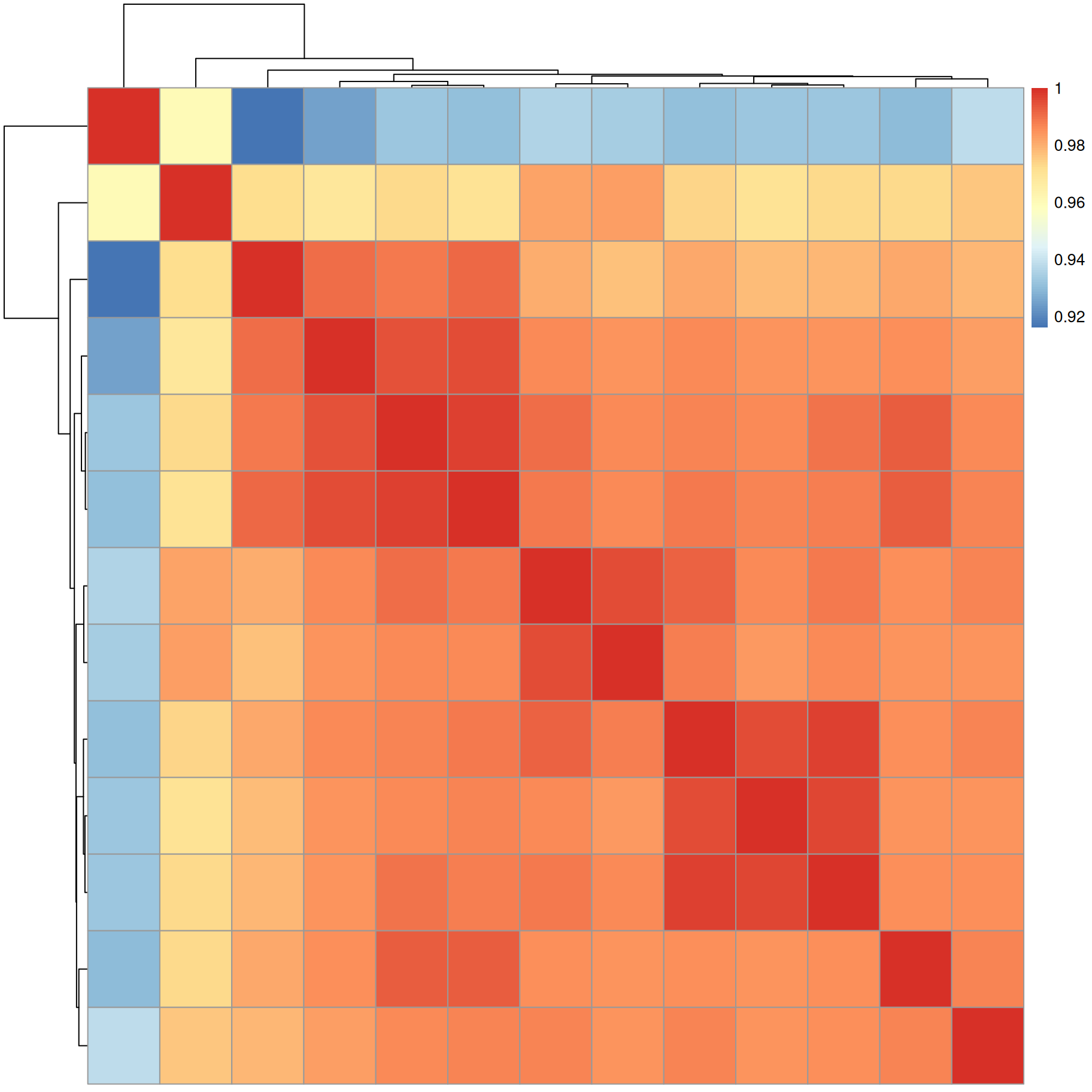
Similarity between all MS2 spectra is very high (above 0.92).
We next combine the individual MS2 spectra of a feature to a single consensus spectrum.
ℹ️ Options to combine spectra
Multiple spectra can be combined into a single spectrum using the
combineSpectra()function which provides a large number of options and parameters for this task, including the possibility to provide a custom function to combine the fragment peaks. By default (with parameterpeaks = "union"), the combined spectrum contains all mass peaks of all input spectra. The optionpeaks = "intersect"allows to retain only peaks that are present in a certain proportion of input spectra. Parametersppmandtolerancedefine the required similarity in the peaks’ m/z value to be considered the same. The groups of spectra to be combined are specified with parameterfand a potential splitting of the inputSpectraobject for parallel processing with parameterp.
As an example, we combine MS2 spectra keeping only mass peaks present in at least 75% of input spectra.
#' define consensus spectra per feature
ms2_cons <- combineSpectra(ms2, f = ms2$feature_id,
                           p = rep(1, length(ms2)),
                           peaks = "intersect",
                           ppm = 10, minProp = 0.75)
ms2_cons
MSn data (Spectra) with 3091 spectra in a MsBackendMemory backend:
msLevel rtime scanIndex
<integer> <numeric> <integer>
1 2 169.3607 834
2 2 147.8949 725
3 2 35.3421 164
4 2 836.9768 4221
5 2 310.3339 1548
... ... ... ...
3087 2 610.293 3053
3088 2 608.046 3050
3089 2 794.229 3958
3090 2 744.275 3673
3091 2 749.801 3791
... 43 more variables/columns.
Processing:
Filter: select retention time [20..850] on MS level(s) [Thu Jul 2 09:29:56 2026]
Filter: select MS level(s) 2 [Thu Jul 2 09:36:18 2026]
Filter: select MS level(s) 2 [Thu Jul 2 09:36:21 2026]
...4 more processings. Use 'processingLog' to list all. We have thus now one consensus spectrum per feature. A summary of the numbers of peaks per consensus spectrum is shown below.
   0%   25%   50%   75%  100%
  1.0  66.5 102.0 146.0 463.0
The consensus spectrum for the first feature is shown below.
plotSpectra(ms2_cons[1], lwd = 2)
grid()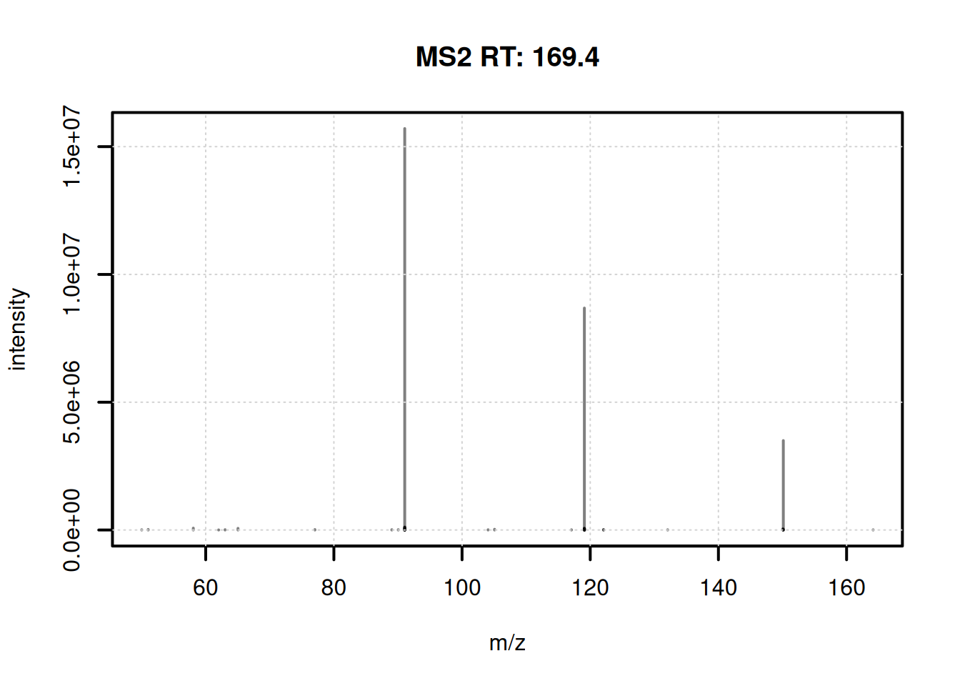
We next filter the data and remove spectra with a single fragment peak.
#' remove spectra with a single fragment peak
ms2_cons <- ms2_cons[lengths(ms2_cons) > 1]
ms2_cons
MSn data (Spectra) with 3089 spectra in a MsBackendMemory backend:
msLevel rtime scanIndex
<integer> <numeric> <integer>
1 2 169.3607 834
2 2 147.8949 725
3 2 35.3421 164
4 2 836.9768 4221
5 2 310.3339 1548
... ... ... ...
3085 2 610.293 3053
3086 2 608.046 3050
3087 2 794.229 3958
3088 2 744.275 3673
3089 2 749.801 3791
... 43 more variables/columns.
Processing:
Filter: select retention time [20..850] on MS level(s) [Thu Jul 2 09:29:56 2026]
Filter: select MS level(s) 2 [Thu Jul 2 09:36:18 2026]
Filter: select MS level(s) 2 [Thu Jul 2 09:36:21 2026]
...4 more processings. Use 'processingLog' to list all. ℹ️ Additional spectra processing options
The Spectra package would provide many additional functions and options to process, scale or clean spectra. As an alternative, through the SpectriPy package, it would also be possible to apply Python-based functionality from e.g. the matchms Python library to
Spectraobjects (Graeve et al. 2025).
At last we visualize the select data (i.e. features with associated MS2 spectra) in the m/z - retention time space. We use the featureArea() function to get the feature boundaries and draw them as rectangles. The associated MS2 spectra (their precursor m/z and retention time value) are added as individual data points.
#' define the feature boundaries
fa <- featureArea(mse, features = ms2_cons$feature_id)

#' plot feature areas as rectangles
plot(NA, NA, xlim = range(fa[, c("rtmin", "rtmax")]),
     ylim = range(fa[, c("mzmin", "mzmax")]),
     xlab = "retention time", ylab = "m/z")
grid()
rect(xleft = fa[, "rtmin"], xright = fa[, "rtmax"],
     ybottom = fa[, "mzmin"], ytop = fa[, "mzmax"],
     border = "#00000080")
#' add precursor m/z and retention times of MS2
points(ms2_cons$rtime, ms2_cons$precursorMz,
       cex = 0.5, col = "#0000ff40")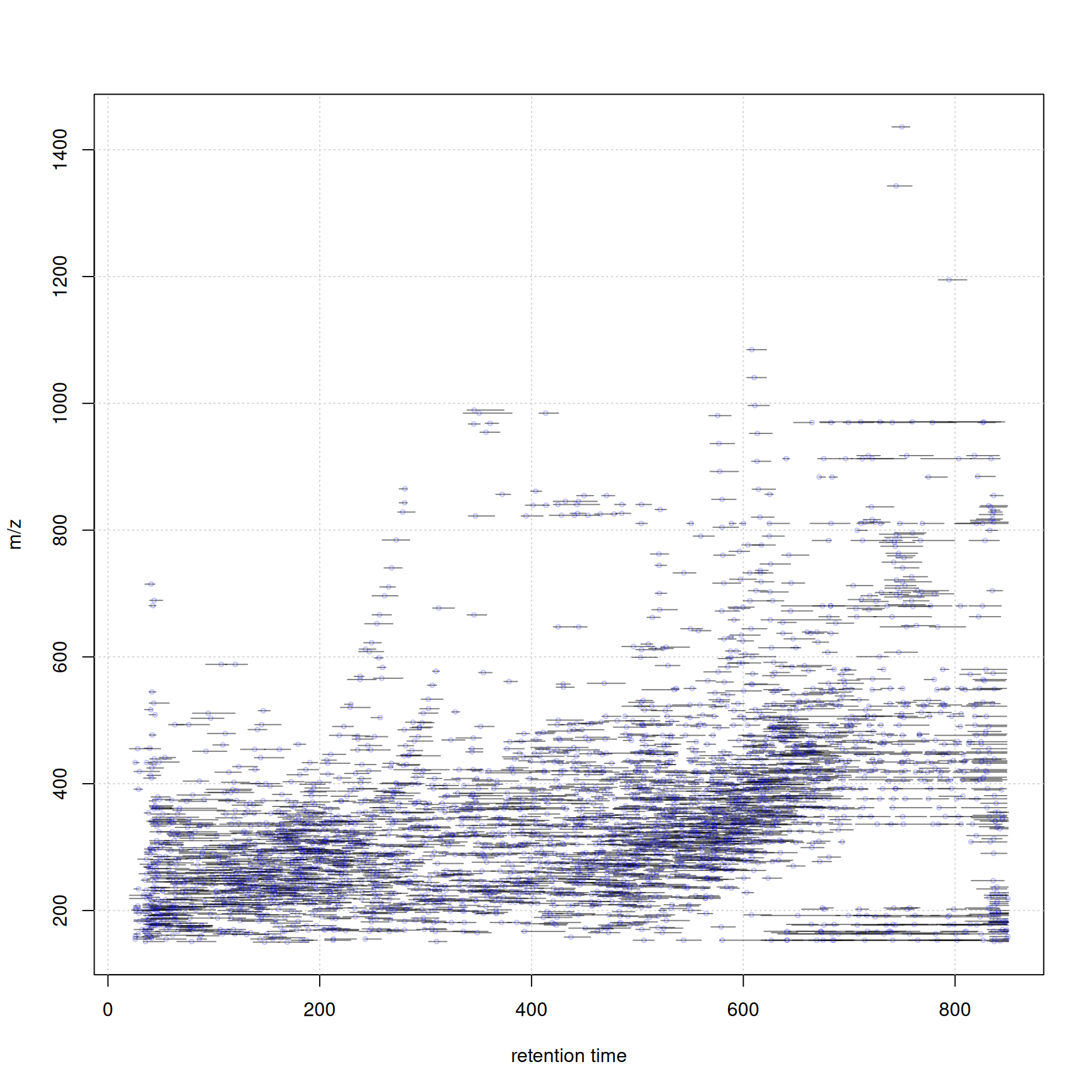
Thus, with a little bit of R coding we can easily create customized data visualizations.
Formatting and exporting data for FBMN
We next export the feature abundance matrix and the fragment spectra for feature-based molecular networking with GNPS. Similar to the original workflow (Rainer and Louail 2025) described in (Nothias et al. 2020) we write the feature matrix to a tabulator delimited text file and the associated MS2 spectra to a file in Mascot Generic File (MGF) format. A future version of the workflow might use the mzTab-M format for the data exchange.
We first compile the feature abundance matrix and export that to a txt file.
#' get feature definitions
fdef <- featureDefinitions(mse)[, c("mzmed", "mzmin", "mzmax",
                                    "rtmed", "rtmin", "rtmax")]
#' combine with the feature value table
fvals <- cbind(Row.names = rownames(fdef), fdef, fvals)

#' restrict the feature abundance matrix to features with MS2 spectra
fvals <- fvals[ms2_cons$feature_id, ]

#' export the data
write.table(fvals, "xcms_ms2_features.txt", sep = "\t",
            quote = FALSE, row.names = FALSE)
We next reformat the information in the MS2 spectra restricting to data required by GNPS. The respective functionality is at present provided in the xcms-gnps-tools GitHub repo.
#' load functions for GNPS-specific spectra formatting
source("https://raw.githubusercontent.com/jorainer/xcms-gnps-tools/master/customFunctions.R")
ms2_cons <- formatSpectraForGNPS(ms2_cons)
And finally we export the consensus MS2 spectra in MGF format.
#' export the MS2 spectra in MGF format
export(ms2_cons, backend = MsBackendMgf(),
       file = "xcms_consensus_ms2_spectra.mgf")
For completeness, we also export all the individual original MS2 spectra to a file xcms_all_ms2_spectra.mgf.
#' export the MS2 spectra in MGF format
setBackend(ms2, MsBackendMemory()) |>
    formatSpectraForGNPS() |>
    export(backend = MsBackendMgf(),
           file = "xcms_all_ms2_spectra.mgf")
ℹ️ Spectra data export formats
The MGF format is only loosely defined with many different dialects being used. The MsBackendMgf package supports renaming or specifying spectra variables (metadata) for export to the MGF format. In addition, it would also allow to export also additional peak information, such as chemical formulas for individual fragments. As an alternative, also other export formats would be supported for
Spectraobjects, provided by packages such as the MsBackendMsp or MsBackendMassbank. Upcoming formats, such as specLib, mzPeak or the updated mzTab-M format will be supported in future.
Summary
- R-based data analysis workflows allow data set specific, tailored, analysis of LC-MS data.
- The xcms R package for LC-MS data preprocessing is tightly integrated into a broader ecosystem of R packages.
- The quarto system would also allow combining R and Python functionality into the same workflow document with the SpectriPy R-package translating between R and Python MS data structures (Graeve et al. 2025).
Session information
The R version and package versions used:
R version 4.6.0 (2026-04-24)
Platform: x86_64-pc-linux-gnu
Running under: Ubuntu 24.04.4 LTS

Matrix products: default
BLAS:   /usr/lib/x86_64-linux-gnu/openblas-pthread/libblas.so.3
LAPACK: /usr/lib/x86_64-linux-gnu/openblas-pthread/libopenblasp-r0.3.26.so;  LAPACK version 3.12.0

locale:
 [1] LC_CTYPE=en_US.UTF-8       LC_NUMERIC=C
 [3] LC_TIME=en_US.UTF-8        LC_COLLATE=en_US.UTF-8
 [5] LC_MONETARY=en_US.UTF-8    LC_MESSAGES=en_US.UTF-8
 [7] LC_PAPER=en_US.UTF-8       LC_NAME=C
 [9] LC_ADDRESS=C               LC_TELEPHONE=C
[11] LC_MEASUREMENT=en_US.UTF-8 LC_IDENTIFICATION=C

time zone: Etc/UTC
tzcode source: system (glibc)

attached base packages:
[1] stats4    stats     graphics  grDevices utils     datasets  methods
[8] base

other attached packages:
 [1] vioplot_0.5.1           zoo_1.8-15              sm_2.2-6.0
 [4] pheatmap_1.0.13         pander_0.6.6            RColorBrewer_1.1-3
 [7] MsBackendMgf_1.20.0     MsBackendMassIVE_0.99.1 xcms_4.10.0
[10] Spectra_1.22.2          BiocParallel_1.46.0     S4Vectors_0.50.1
[13] BiocGenerics_0.58.1     generics_0.1.4          MsExperiment_1.14.0
[16] ProtGenerics_1.44.0

loaded via a namespace (and not attached):
  [1] DBI_1.3.0                   httr2_1.2.3
  [3] rlang_1.2.0                 magrittr_2.0.5
  [5] clue_0.3-68                 MassSpecWavelet_1.78.0
  [7] otel_0.2.0                  matrixStats_1.5.0
  [9] compiler_4.6.0              RSQLite_3.53.3
 [11] PTMods_1.0.0                vctrs_0.7.3
 [13] reshape2_1.4.5              rvest_1.0.5
 [15] stringr_1.6.0               pkgconfig_2.0.3
 [17] MetaboCoreUtils_1.20.1      crayon_1.5.3
 [19] fastmap_1.2.0               dbplyr_2.6.0
 [21] XVector_0.52.0              rmarkdown_2.31
 [23] preprocessCore_1.74.0       bit_4.6.0
 [25] purrr_1.2.2                 xfun_0.59
 [27] MultiAssayExperiment_1.38.0 cachem_1.1.0
 [29] jsonlite_2.0.0              progress_1.2.3
 [31] blob_1.3.0                  DelayedArray_0.38.2
 [33] parallel_4.6.0              prettyunits_1.2.0
 [35] cluster_2.1.8.2             R6_2.6.1
 [37] stringi_1.8.7               limma_3.68.4
 [39] GenomicRanges_1.64.0        Rcpp_1.1.1-1.1
 [41] Seqinfo_1.2.0               SummarizedExperiment_1.42.0
 [43] iterators_1.0.14            knitr_1.51
 [45] IRanges_2.46.0              Matrix_1.7-5
 [47] igraph_2.3.3                tidyselect_1.2.1
 [49] abind_1.4-8                 yaml_2.3.12
 [51] doParallel_1.0.17           codetools_0.2-20
 [53] affy_1.90.0                 curl_7.1.0
 [55] lattice_0.22-9              tibble_3.3.1
 [57] plyr_1.8.9                  withr_3.0.3
 [59] Biobase_2.72.0              S7_0.2.2
 [61] evaluate_1.0.5              BiocFileCache_3.2.0
 [63] xml2_1.6.0                  filelock_1.0.3
 [65] pillar_1.11.1               affyio_1.82.0
 [67] BiocManager_1.30.27         MatrixGenerics_1.24.0
 [69] foreach_1.5.2               MSnbase_2.37.0
 [71] MALDIquant_1.22.3           ncdf4_1.24
 [73] hms_1.1.4                   ggplot2_4.0.3
 [75] scales_1.4.0                glue_1.8.1
 [77] MsFeatures_1.20.0           lazyeval_0.2.3
 [79] tools_4.6.0                 mzID_1.50.0
 [81] data.table_1.18.4           QFeatures_1.22.0
 [83] vsn_3.80.0                  mzR_2.46.0
 [85] fs_2.1.0                    XML_3.99-0.23
 [87] grid_4.6.0                  impute_1.86.0
 [89] tidyr_1.3.2                 MsCoreUtils_1.24.0
 [91] PSMatch_1.16.0              cli_3.6.6
 [93] rappdirs_0.3.4              S4Arrays_1.12.0
 [95] dplyr_1.2.1                 AnnotationFilter_1.36.0
 [97] pcaMethods_2.4.0            gtable_0.3.6
 [99] digest_0.6.39               SparseArray_1.12.2
[101] farver_2.1.2                memoise_2.0.1
[103] htmltools_0.5.9             lifecycle_1.0.5
[105] httr_1.4.8                  statmod_1.5.2
[107] bit64_4.8.2                 MASS_7.3-65
References
Graeve, Marilyn De, Wout Bittremieux, Thomas Naake, et al. 2025. “SpectriPy: Enhancing Cross-Language Mass Spectrometry Data Analysis with R and Python.” Journal of Open Source Software 10 (109): 8070. https://doi.org/10.21105/joss.08070.
Louail, Philippine, Carl Brunius, Mar Garcia-Aloy, et al. 2025. “Xcms in Peak Form: Now Anchoring a Complete Metabolomics Data Preprocessing and Analysis Software Ecosystem.” Analytical Chemistry, ahead of print, December. https://doi.org/10.1021/acs.analchem.5c04338.
Louail, Philippine, Marilyn De Graeve, Anna Tagliaferri, Vinicius Verri Hernandes, Daniel Marques de Sá e Silva, and Johannes Rainer. 2025. Rformassspectrometry/Metabonaut: V1.2.0. Zenodo. https://doi.org/10.5281/zenodo.15554287.
Nothias, Louis-Félix, Daniel Petras, Robin Schmid, et al. 2020. “Feature-Based Molecular Networking in the GNPS Analysis Environment.” Nature Methods 17 (9): 905–8. https://doi.org/10.1038/s41592-020-0933-6.
Rainer, Johannes, and Philippine Louail. 2025. Jorainer/Xcms-Gnps-Large-Scale: Preprocessing of a Large LC-MS/MS Data Set for Molecular Networking with GNPS. V. v1.0.0. Zenodo, released October. https://doi.org/10.5281/zenodo.17293665.